R Users’ Salaries from the 2019 Stackoverflow Survey
Let’s take a look on what R users are saying about their salaries. Note that the following results could be biased because of unrepresentative and in some cases small samples.
By Tomaž Weiss, Data Scientist
Introduction
Stackoverflow has recently released the anonymized results of their 2019 annual developer survey. Let’s take a look on what R users are saying about their salaries. Note that the following results could be biased because of unrepresentative and in some cases small samples.
Data Preparation
The dataset consists of survey answers from nearly 90,000 respondents. About 5,000 of them reported using R for “extensive development work over the past year”.
We first import the data and keep only the respondents who use R as part of their professional work.
library(tidyverse)
library(countrycode)

# data import -------------------------------------------------------------

data <- read_csv("data/survey_results_public.csv")

# data preparation -----------------------------------------------------------

data_r <-
  data %>%
  filter(grepl('^R$', LanguageWorkedWith) | grepl(';R$', LanguageWorkedWith) |
           grepl(';R;', LanguageWorkedWith) | grepl('^R;', LanguageWorkedWith)) %>%
  filter(MainBranch %in% c('I am a developer by profession',
                           'I am not primarily a developer, but I write code sometimes as part of my work')) %>%
  filter(Employment %in% c('Employed full-time',
                           'Employed part-time',
                           'Independent contractor, freelancer, or self-employed')) %>%
  filter(!grepl('Other Country', Country)) %>%
  filter(!is.na(Country), !is.na(ConvertedComp), ConvertedComp > 0)
The first filter used reduces the dataset from 88,883 respondents to 5,048. The second filter excludes students, hobby programmers and former developers. This reduces the dataset to 4,047 respondents. The third filter excludes unemployed and retired respondents and the dataset is further reduced to 3,871 respondents. Finally, we exclude respondents from an unknown country and respondents with unknown or zero salary (variable ConvertedComp). The final dataset size is 3,034 rows (respondents).
We need two additional helper tables. The first one will contain number of R users and their median annual USD salary by country.
# number of respondents using R by country
country_n_r_users <-
  data_r %>%
  group_by(Country) %>%
  summarise(n_r_users = n(), median_convertedcomp = round(median(ConvertedComp)))

country_n_r_users %>% arrange(desc(n_r_users))
## # A tibble: 109 x 3
##    Country        n_r_users median_convertedcomp
##    <chr>              <int>                <dbl>
##  1 United States       1100               110000
##  2 Germany              197                61872
##  3 United Kingdom       190                68695
##  4 India                149                10920
##  5 Canada               105                64888
##  6 Netherlands           85                54996
##  7 France                81                41247
##  8 Brazil                80                16062
##  9 Australia             79                78332
## 10 Spain                 64                32254
## # ... with 99 more rows
The second table will contain country-continent information. We can use the handy countrycode::countrycode function for this task:
# country - continent table
countries <-
  data %>%
  filter(!grepl('Other Country', Country)) %>%
  distinct(Country) %>%
  mutate(continent = countrycode(sourcevar = Country, origin = "country.name", destination = "continent"))

countries
## # A tibble: 179 x 2
##    Country                continent
##    <chr>                  <chr>
##  1 United Kingdom         Europe
##  2 Bosnia and Herzegovina Europe
##  3 Thailand               Asia
##  4 United States          Americas
##  5 Ukraine                Europe
##  6 Canada                 Americas
##  7 India                  Asia
##  8 New Zealand            Oceania
##  9 Antigua and Barbuda    Americas
## 10 Germany                Europe
## # ... with 169 more rows
Salary Distributions by Country
Our variable of interest is called ConvertedComp and is defined as “salary converted to annual USD salaries using the exchange rate on 2019-02-01, assuming 12 working months and 50 working weeks.”
Annual salary distributions are visualized below by boxplots. To avoid displaying (too much) noise, we limit ourselves to countries with at least five reported R users.
# boxplot visualization ---------------------------------------------------

data_r %>%
  left_join(countries, by = "Country") %>%
  inner_join(country_n_r_users %>% filter(n_r_users >= 5), by = "Country") %>%
  mutate(Country = reorder(Country, ConvertedComp, median)) %>%
  ggplot(aes(x = Country, y = ConvertedComp, fill = continent)) +
  geom_boxplot(outlier.size = 0.5) +
  ylab('Annual USD salary') +
  coord_flip(ylim = c(0, 200000)) +
  scale_y_continuous(breaks = seq(0, 200000, by = 20000),
                     labels = function(x) format(x, big.mark = ",", decimal.mark = '.', scientific = FALSE)
                     ) +
  ggtitle("Distributions of R Users' Salaries by Country") +
  theme(plot.title = element_text(hjust = 0.5)) +
  scale_fill_discrete(name = "Continent")
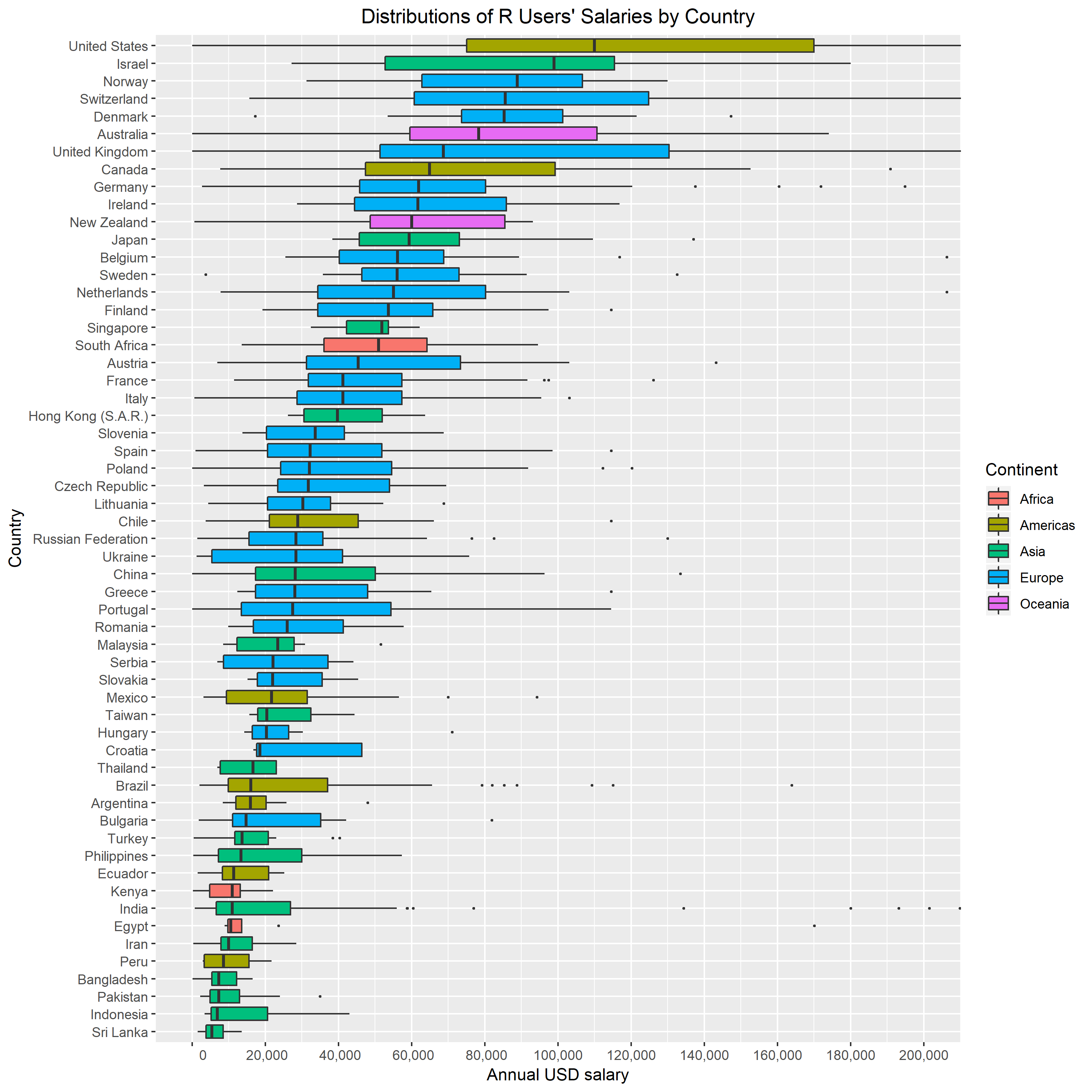
United States has the highest median annual salary at 110,000 USD, followed by Israel and Norway. The lower part of the graph is populated by Asian, South American and African countries.
Salary Distributions for United States
Let’s have a quick look at R users’ salary distributions by some interesting variables for country with the highest number of respondents (1,100).
Age
# Age
data_r %>%
  filter(Country == 'United States') %>%
  filter(!is.na(Age)) %>%
  filter(Age >= 20) %>%
  ggplot(aes(x = as.factor(floor(Age/10)), y = ConvertedComp)) +
  geom_boxplot(outlier.shape = NA) +
  coord_cartesian(ylim = c(0, 300000)) +
  geom_jitter(aes(as.factor(floor(Age/10)), ConvertedComp),
              position = position_jitter(width = 0.1, height = 0),
              alpha = 0.6,
              size = 1) +
  scale_y_continuous(breaks = seq(0, 300000, by = 20000),
                     labels = function(x) format(x, big.mark = ",", decimal.mark = '.', scientific = FALSE)
                     ) +
  ylab('Annual USD salary') +
  xlab('Age bin (years)') +
  ggtitle("Distributions of R Users' Salaries by Age Bin for United States") +
  theme(plot.title = element_text(hjust = 0.5)) +
  scale_x_discrete(labels=c("2" = "20-29", "3" = "30-39",
                          "4" = "40-49", "5" = "50-59", "6" = "60-69"))

The median of the second age group is is about 40% higher than the median of the first one. The median of the third age group is is about 17% higher than the median of the second one. The median of the fourth age group is is about 6% higher than the median of the third one. Note that a few respondents reported salaries very close to zero.
Gender
Similarly, distributions by gender can be plotted:
# Gender
data_r %>%
  filter(Country == 'United States') %>%
  filter(!is.na(Gender)) %>%
  mutate(Gender = if_else(Gender %in% c('Man', 'Woman'), Gender, 'Other')) %>%
  mutate(Gender = reorder(Gender, ConvertedComp, median)) %>%
  ggplot(aes(x = as.factor(Gender), y = ConvertedComp)) +
  geom_boxplot(outlier.shape = NA) +
  coord_cartesian(ylim = c(0, 300000)) +
  geom_jitter(aes(as.factor(Gender), ConvertedComp),
              position = position_jitter(width = 0.1, height = 0),
              alpha = 0.6,
              size = 1) +
  scale_y_continuous(breaks = seq(0, 300000, by = 20000),
                     labels = function(x) format(x, big.mark = ",", decimal.mark = '.', scientific = FALSE)
                     ) +
  ylab('Annual USD salary') +
  xlab('Gender') +
  ggtitle("Distributions of R Users' Salaries by Gender for United States") +
  theme(plot.title = element_text(hjust = 0.5))

Men report to earn about 15% higher median salary than women.
Education Level
Rare education categories are excluded here for better readability.
# EdLevel
data_r %>%
  filter(Country == 'United States') %>%
  filter(!is.na(EdLevel)) %>%
  inner_join(
    data_r %>%
      filter(Country == 'United States') %>%
      filter(!is.na(EdLevel)) %>%
      group_by(EdLevel) %>%
      count() %>%
      filter(n >= 20) %>%
      select(EdLevel),
    by = 'EdLevel'
  ) %>%
  mutate(EdLevel = reorder(EdLevel, ConvertedComp, median)) %>%
  ggplot(aes(x = EdLevel, y = ConvertedComp)) +
  geom_boxplot(outlier.shape = NA) +
  theme(axis.text.x = element_text(angle = 60, hjust = 1)) +
  geom_jitter(aes(EdLevel, ConvertedComp),
              position = position_jitter(width = 0.1, height = 0),
              alpha = 0.6,
              size = 1) +
  scale_y_continuous(breaks = seq(0, 300000, by = 20000),
                     labels = function(x) format(x, big.mark = ",", decimal.mark = '.', scientific = FALSE)) +
  coord_flip(ylim = c(0, 300000)) +
  ylab('Annual USD salary') +
  xlab('Education Level') +
  ggtitle("Distributions of R Users' Salaries by Education Level for United States") +
  theme(plot.title = element_text(hjust = 0.5))

Bachelor’s degree holders report earning about 15% more than respondents without a degree (median difference). Master’s degree holders report earning about 9% more than respondents with bachelor’s degree. Ph.D. holders report earning about 18% more than respondents with master’s degree.
Undergraduate Major
R users come from a diverse set of undergraduate degrees. Again we exclude rare majors.
# UndergradMajor
data_r %>%
  filter(Country == 'United States') %>%
  filter(!is.na(UndergradMajor)) %>%
  inner_join(
    data_r %>%
      filter(Country == 'United States') %>%
      filter(!is.na(UndergradMajor)) %>%
      group_by(UndergradMajor) %>%
      count() %>%
      filter(n >= 10) %>%
      select(UndergradMajor),
    by = 'UndergradMajor'
  ) %>%
  mutate(UndergradMajor = reorder(UndergradMajor, ConvertedComp, median)) %>%
  ggplot(aes(x = UndergradMajor, y = ConvertedComp)) +
  geom_boxplot(outlier.shape = NA) +
  theme(axis.text.x = element_text(angle = 45, hjust = 1)) +
  geom_jitter(aes(UndergradMajor, ConvertedComp),
              position = position_jitter(width = 0.1, height = 0),
              alpha = 0.6,
              size = 1) +
  scale_y_continuous(breaks = seq(0, 300000, by = 20000),
                     labels = function(x) format(x, big.mark = ",", decimal.mark = '.', scientific = FALSE)) +
  coord_flip(ylim = c(0, 300000)) +
  ylab('Annual USD salary') +
  xlab('Undergraduate Major') +
  ggtitle("Distributions of R Users' Salaries by Undergraduate Major for US") +
  theme(plot.title = element_text(hjust = 0.5))
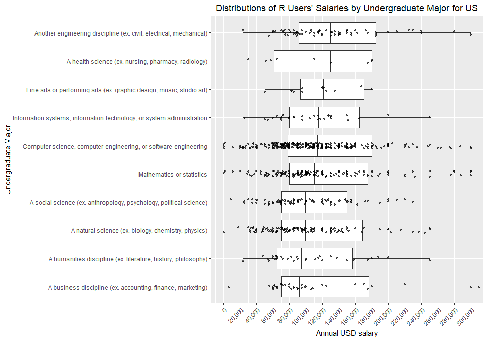
Interestingly, the highest median salary is reported by “other” engineering majors (civil, electrical, mechanical).
Developer Type
Note that each survey respondent had an option to pick more than one category here. Even though we removed students from the MainBranch column at the beginning of the analysis, some developers still report being a student in the DevType column.
# DevType
data_r %>%
  filter(Country == 'United States') %>%
  filter(!is.na(DevType)) %>%
  select(Respondent, ConvertedComp, DevType) %>%
  mutate(DevType_ = str_split(DevType, ';')) %>%
  unnest() %>%
  select(-DevType) %>%
  mutate(DevType = reorder(DevType_, ConvertedComp, median)) %>%
  ggplot(aes(x = DevType, y = ConvertedComp)) +
  geom_boxplot(outlier.shape = NA) +
  coord_flip(ylim = c(0, 350000)) +
  theme(axis.text.x = element_text(angle = 45, hjust = 1)) +
  geom_jitter(aes(DevType, ConvertedComp),
              position = position_jitter(width = 0.1, height = 0),
              alpha = 0.6,
              size = 1) +
  scale_y_continuous(breaks = seq(0, 350000, by = 20000),
                     labels = function(x) format(x, big.mark = ",", decimal.mark = '.', scientific = FALSE)) +
  ylab('Annual USD salary') +
  xlab('Developer Type') +
  ggtitle("Distributions of R Users' Salaries by Developer Type for United States") +
  theme(plot.title = element_text(hjust = 0.5))

As expected, executives and managers earn the most and students earn the least.
Conclusion
I hope you found the above insights interesting. Feel free to experiment with this data by yourself and share your findings.
Session Info
sessionInfo()
## R version 3.5.3 (2019-03-11)
## Platform: x86_64-w64-mingw32/x64 (64-bit)
## Running under: Windows 10 x64 (build 17763)
##
## Matrix products: default
##
## locale:
## [1] LC_COLLATE=Slovenian_Slovenia.1250  LC_CTYPE=Slovenian_Slovenia.1250
## [3] LC_MONETARY=Slovenian_Slovenia.1250 LC_NUMERIC=C
## [5] LC_TIME=Slovenian_Slovenia.1250
##
## attached base packages:
## [1] stats     graphics  grDevices utils     datasets  methods   base
##
## other attached packages:
##  [1] countrycode_1.1.0 forcats_0.4.0     stringr_1.4.0
##  [4] dplyr_0.8.0.1     purrr_0.3.2       readr_1.3.1
##  [7] tidyr_0.8.3       tibble_2.1.1      ggplot2_3.1.1
## [10] tidyverse_1.2.1
##
## loaded via a namespace (and not attached):
##  [1] Rcpp_1.0.1       cellranger_1.1.0 pillar_1.3.1     compiler_3.5.3
##  [5] plyr_1.8.4       tools_3.5.3      digest_0.6.18    lubridate_1.7.4
##  [9] jsonlite_1.6     evaluate_0.13    nlme_3.1-137     gtable_0.3.0
## [13] lattice_0.20-38  pkgconfig_2.0.2  rlang_0.3.4      cli_1.1.0
## [17] rstudioapi_0.10  yaml_2.2.0       haven_2.1.0      xfun_0.6
## [21] withr_2.1.2      xml2_1.2.0       httr_1.4.0       knitr_1.22
## [25] hms_0.4.2        generics_0.0.2   grid_3.5.3       tidyselect_0.2.5
## [29] glue_1.3.1       R6_2.4.0         fansi_0.4.0      readxl_1.3.1
## [33] rmarkdown_1.12   modelr_0.1.4     magrittr_1.5     backports_1.1.4
## [37] scales_1.0.0     htmltools_0.3.6  rvest_0.3.2      assertthat_0.2.1
## [41] colorspace_1.4-1 utf8_1.1.4       stringi_1.4.3    lazyeval_0.2.2
## [45] munsell_0.5.0    broom_0.5.2      crayon_1.3.4
Bio: Tomaž Weiss is a Data Scientist from Ljubljana, Slovenia.
Original. Reposted with permission.
Related:
- Ten more random useful things in R you may not know about
- What does a data scientist REALLY look like?
- Data Scientists: Why are they so expensive to hire?