


The FIFA World Cup ended nearly a month ago, and we can now bring down the curtain on a memorable season with its fair share of emotions and surprises. Sadly, our favorite team didn’t win, but it’s not a big deal since the model we created to predict World Cup game outcomes performed very well! If you haven’t heard about how we used ML to make 2022 World Cup predictions, we invite you to check our first blog post here, as there will be many references to what we previously detailed.
In this blog post, you will learn how we used Dataiku to develop another strategy and make predictions. We will also compare the different approaches and their results, and you will get a better idea of the challenges we faced when implementing these models. The first part of the article is intended for rather technical practitioners, while the results analysis part will be more accessible.
Traditional ML vs. Poisson Regression
The first blog post presented a “traditional” ML approach. Here, we will consider a probabilistic approach, with stronger assumptions but one that results in a more interpretable (and simpler) model.
Assumption on the Target Variable
The Poisson distribution is a discrete probability distribution that expresses the probability of a given number of events that occur in a fixed interval of time or space if these events occur with a known constant mean rate (λ) and independently of the time since the last event. A Poisson distribution, with parameter λ > 0, has a probability mass function given by
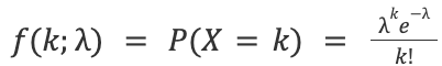
with the property that the mean equals λ.
In our case, goals scored by each team are assumed to be Poisson distributed with the mean rate (λ) representing the expected goals within 90 minutes (the scoring intensity). A goal can occur at any moment in the match in a totally random way, with no dependencies on previous goals. We are aware that assumption might be seen as unrealistic, but naturally we tend to start with strong assumptions and relax them gradually.
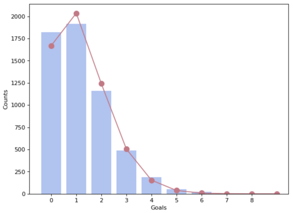
Distribution of goals on the entire dataset (in blue the distribution observed on the dataset, in red the theoretical Poisson one).
A famous regression model for count data is the Poisson regression model which is a generalized linear model (GLM) form. GLM is a flexible version of the OLS (Ordinary Least Squares) that allows:
- The response Y to be non-normal, but from a more general type of distribution (“one-parameter exponential” family)
- The linear model to be related to the response variable via a link function.
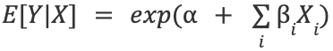
Poisson regression assumes the response variable Y has a Poisson distribution and the logarithm of its expected value can be modeled by a linear combination of explanatory variables:

with 𝛂 the intercept, 𝛃i the regression coefficients and Xi the input variables. And so
with the coefficients determined using the MLE (Maximum Likelihood Estimator).
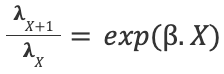
For a unit change in the input variable X, we will have a percent change in the response represented by the following rate ratio:
In our case, the scoring intensity λ is assumed to be explained as a combination of latent parameters representing teams' attack and defense abilities/strengths, and can be enriched with team specific and other features. This assumption is made to have the scores of the two teams treated independently from each other. Indeed, the score of team A depends on team A’s offensive ability and team B’s defensive ability (and other effects), and vice versa for team B: The explanatory variables for the two scores in a match are distinct from each other, which ensure independence between the scores.
Model Output
The model returns the expected average number of goals λ for each team in a match, meaning we can calculate the probability over goals with the Poisson distribution formula. With the independence between the two scores, the probability for any match scoreline is derived by taking the product of the two probabilities.
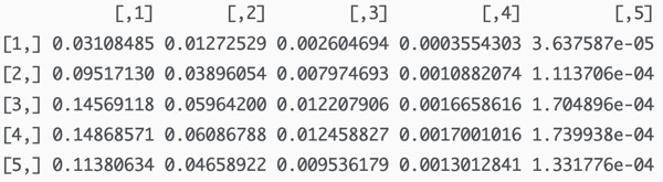
Matrix showing the probability on the possible scorelines (rows correspond to the score of team A, columns to team B)
From this, we can derive the probability of various events. For example, the probability of a draw is simply the sum of the events where the two teams score the same amount of goals.
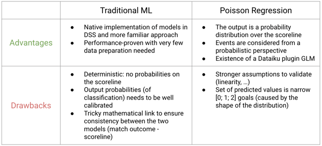
The table below summarizes the advantages and drawbacks of the two strategies:
Now let’s reveal the final results!
Results and Analysis
How Did the Models Perform?
One of the great things about these World Cup predictions is that we’ve been able, after just one month of competition, to compare our predictions with what really happened during the 64 games, and conduct post-hoc analysis on how our model performed.
Before diving deeper into the performances of our models, let’s define the baseline that we used. We considered the baseline performance as the minimum goal to reach in order for machine learning (ML) to be worth using. We used a quite straightforward baseline, consisting of simply going for the most likely outcome (the one with the smallest odds) for each game. There is no ML involved with this baseline, it is just about using the odds of the bookmaker and selecting the favorite outcome.
After defining this baseline, we used three different strategies that we mentioned above and in the first blog post. Let’s give a quick reminder.
Using the traditional ML approach:
- A basic strategy: This one is quite straightforward, as the selected outcome (Win / Draw / Lose) is simply the one with the highest predicted probability by the classification model (i.e., the most likely one).
- A gain optimization strategy: We compute the potential gain associated with each outcome (given by the formula outcome probability * outcome odds), and select the outcome with the highest potential gain (you can refer to the France vs. Australia example detailed in the first blog post).
Using the Poisson regression approach:
- A gain optimization strategy: same as above
Let’s now review the performances of these three strategies. We will consider three metrics:
- The number of correctly predicted games (games for which we predicted the correct outcome)
-
The number of points earned (the sum of the outcome odds for games correctly predicted)
- >The final return, i.e., the total points normalized by the number of games. This can give you an idea of how much money you would have made if you had bet the same amount of money on each game.
Here is a table that summarizes the performances of three strategies that we conducted.
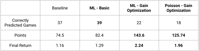
A few interesting takeaways from this table:
1. The baseline strategy, even if it’s very simple, does yield some positive results (return > 1), and correctly predicts a majority of outcomes (37 / 64).
2. Even with this baseline being not bad at all, our basic strategy using traditional ML did outperform it, correctly predicting a higher number of games! So this shows that ML is worth using in that case, and can yield better results than just looking at the odds and betting on the favorite (a ratio of 1.29 means a 29% return on your money, so quite interesting).
That was a first achievement for us.
3. Even more interesting, the gain optimization strategy materially outperformed the baseline. Indeed, even with fewer correct predictions, the odds of the correct predictions were so big (because the bets were risky) that we almost doubled the number of points earned by the baseline! That means a ratio of 2.24, so potentially more than doubling your stake!
These results were good enough to win our social betting contest that involved 250 players among Dataiku employees and our customers with the ML - Gain Optimization strategy 🏆
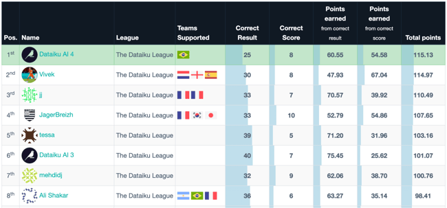
To compare our results on a much larger scale, we can take the ranking of the French reference social betting app MonPetitProno (MPP). Using this ranking, our ML - Gain Optimization strategy would rank ~5,000 out of 1.7 million players, putting us in the top 0.3%. This is an excellent result for a strategy developed in such a short period of time 🥳
Challenges and Limitations
Although our results were very satisfying and beyond expectations, we faced a few challenges and limitations on the road of implementing our strategies.
Probability Calibration
Our very first constraint was probability calibration. In order to win the betting contest, our goal was to maximize the expected gain, which we get by multiplying the predicted probability by the odds. Therefore, we needed our model to predict probability estimates that would be representative of the true likelihood. Hence, the need for probability calibration.
You can find many calibration techniques, the main idea behind them is to fit a smoothing model on the predictions. Some common methods include:
- Platt scaling which assumes a logistic relationship between the predictions and the true probabilities.
- Spline calibration which will fit a smooth cubic polynomial on the predictions
Quantitative metrics such as Expected Calibration Error can be used to assess if our model is well calibrated, but a popular visual method is the Reliability Curve.
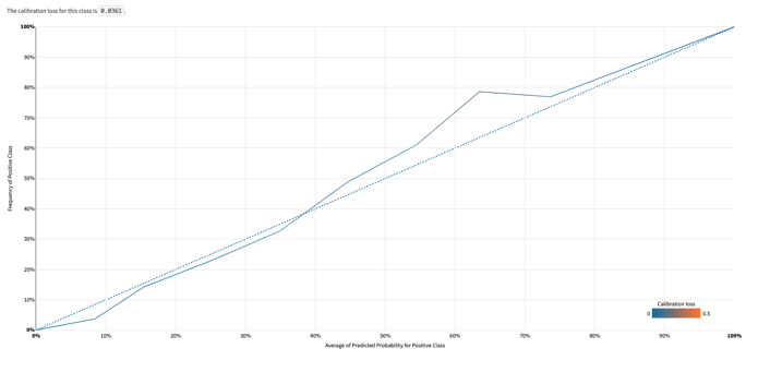
Reliability curve from our Random Forest Classifier predicting games’ outcome
This plot compares the fraction of true positives as a function of the averaged predicted probabilities for different bins. For a perfectly calibrated model, those two values would be equal. Therefore, the closest the curve is to the diagonal identity, the better calibrated our model is.
Consistency of 2-Step Model
Let’s talk about another obstacle we faced. In our traditional approach, we chained two random forest models. The first model’s outcome predictions were fed into the second model that predicted the scoreline. However, there was no guarantee the two models would produce consistent predictions. What if the first model predicts France wins against Argentina, but the second model predicts a score line of 1 - 2 for Argentina? A guard rail is necessary to prevent those situations from happening, whether it is by using post-processing techniques or other modeling strategies.
How Confident Can We Be in Our Model?
Even though our results are great, we need to take a step back to better understand them and assess how robust they are.
- First limitation is the size of the prediction set (64 World Cup matches)
-
Such a sample size does not put us in the law of large numbers. Our result might not be replicable in future World Cups and competitions.
-
On top of that, the smaller the sample is, the wider the confidence interval around our result is.
-
To circumvent this limitation, we can use a resampling method (such as bootstrapping) to create a confidence interval and see where the original result is located.
- Potential drift of the target variable
-
With 172 goals, this edition became the World Cup with most goals in its 92-year-old history. That raises the question of a potential shift in the distribution of goals in this World Cup edition compared to previous competitions.
-
-
Most of the points were brought by very few games
-
Should we consider some extremely rare events — those with the most imbalanced odd ratio — as outliers? The most obvious example is Saudi Arabia beating the future champion and bringing a quarter of the total points for the classical ML model.
-
More broadly, are unlikely match outcomes (“upsets”) over-represented in this competition in comparison with previous ones?
-
To Go Beyond...
So, is it possible to predict sports results using AI? Hard to say “yes,” as there were many unexpected events that happened during this World Cup, but the model was able to do better than all the other human players of the betting contest, so not too bad!
Next time, we could try including other variables such as team composition or historical betting odds or be more fussy when selecting our train/test set to improve our models. See you maybe in four years. Until then, stay well!