Introduction

In this blog post, we will explore the Decoder-Only Transformer architecture, which is a variation of the Transformer model primarily used for tasks like language translation and text generation. The Decoder-Only Transformer consists of several blocks stacked together, each containing key components such as masked multi-head self-attention and feed-forward transformations.

Learning Objectives

•  Explore the architecture and components of the Decoder-Only Transformer model.
• Understand the role of attention mechanisms, including Scaled Dot-Product Attention and Masked Self-Attention, in the model.
•  Examine the importance of positional embeddings and normalization techniques in transformer models.
• Discuss the use of feed-forward transformations and residual connections in improving training stability and efficiency.

Components of Decoder-Only Transformer Blocks

Let’s delve into these components and the overall structure of the model.

Scaled Dot-Product Attention

This is a crucial mechanism within each transformer block, determining attention scores based on token similarity in the sequence. These scores are then utilized to evaluate the significance of each token in generating the output.

Tokens

Understanding attention begins with the input to a self-attention layer, which consists of a batch of token sequences. Each token is represented by a vector in the sequence, assuming a batch size of b and a sequence length of max_len. The self-attention layer receives a tensor of shape [ batch-size, seq_len, token dimensionality ]. 

Self-attention Layer Inputs  

It employs three linear layers for query, key, and value, transforming the input into key, vector, and value sequences. These linear layers involve matrix multiplication with the key, query, and value components.

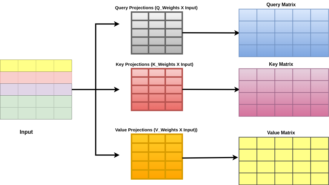
Attention Scores are generated by comparing the key and query vectors. The attention score[i,j] measures the impact of token j on the new representation of token i in a sequence. Scores are computed via dot product of query vector for token i and key vector for token j.

The multiplication of the query with the transposed key matrix yields an attention matrix of size [ seq_len,seq_len ], containing pairwise attention scores in the sequence. Matrix is divided by sqrt(d) for stability, followed by softmax for valid probability distributions.

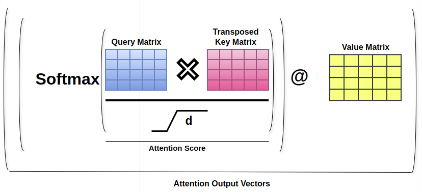
Value Vectors are then determined based on the attention scores, creating a weighted combination of value vectors for each token. Taking the dot product of the attention matrix with the value matrix produces a d-dimensional output vector for each token in the input sequence.

Implementation with Code

import torch
import torch.nn.functional as F

# Assume input tensors
batch_size = 32
seq_len = 10
token_dim = 64
d = token_dim  # Dimensionality of tokens

# Generate random input tensor
input_tensor = torch.randn(batch_size, seq_len, token_dim)
# Linear layers for query, key, and value
query_layer = torch.nn.Linear(token_dim, d)
key_layer = torch.nn.Linear(token_dim, d)
value_layer = torch.nn.Linear(token_dim, d)

# Apply linear transformations
query = query_layer(input_tensor)
key = key_layer(input_tensor)
value = value_layer(input_tensor)

# Compute attention scores
scores = torch.matmul(query, key.transpose(-2, -1))  # Dot product of query and key
scores /= torch.sqrt(torch.tensor(d, dtype=torch.float32))  # Scale by square root of d

# Apply softmax to get attention weights
attention_weights = F.softmax(scores, dim=-1)
# Weighted sum of value vectors based on attention weights
weighted_sum = torch.matmul(attention_weights, value)
print(weighted_sum)

Masked Self-Attention

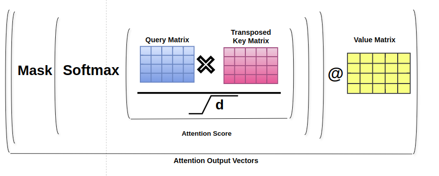
During training, the decoder adjusts self-attention to prevent tokens from attending to future tokens, ensuring autoregressive output generation without information leakage. This modified self-attention, known as masked self-attention, is a variant that selectively includes tokens in the attention computation while excluding future tokens based on their position in the sequence.

Consider a token sequence [‘you’, ‘are’, ‘making’, ‘progress’, ‘.’]. If we focus on computing attention scores for the token ‘are’, masked self-attention only considers tokens preceding ‘making’ in the sequence, such as ‘you’ and ‘are’, while excluding ‘progress’ and ‘.’. This restriction ensures that during self-attention, the model cannot access information from tokens ahead in the sequence.

To implement masked self-attention, after multiplying the query and key matrices, we obtain an attention matrix of size [seq_len, seq_len], containing attention scores for each token pair in the sequence. Before applying the softmax operation row-wise to this matrix, we set all values above the diagonal (representing future tokens) to negative infinity. This manipulation ensures that during softmax, tokens can only attend to previous or current tokens, effectively masking out any information from future tokens. As a result, the attention scores are adjusted to exclude tokens that follow a given token in the sequence.

Attention

The attention mechanism we’ve discussed utilizes softmax to normalize attention scores across the sequence, forming a valid probability distribution. This approach can lead to attention being dominated by a few words. Thus limiting the model’s ability to focus on multiple positions within the sequence. To address this, we divide the attention into multiple heads. Each head performs the masked attention operation independently but with separate key, query, and value projections.

Multiheaded self-attention uses separate projections for each head to reduce computational costs by reducing the dimensionality of key, query, and value vectors from d to d//H, where H represents the number of heads. This allows each head to learn unique representational subspaces and focus on different parts of the sequence, while mitigating computational expenses. The output of each head can be combined through concatenation, averaging, or projection. The concatenated output from all attention heads maintains a dimension of d, the same as the input dimension of the attention layer.

Implementation with Code

import torch
import torch.nn.functional as F

class MultiheadSelfAttention(torch.nn.Module):a
   def __init__(self, d_model, num_heads):
       super(MultiheadSelfAttention, self).__init__()
       assert d_model % num_heads == 0, "d_model must be divisible by num_heads"
       self.d_model = d_model
       self.num_heads = num_heads
       self.head_dim = d_model // num_heads

       self.query_linear = torch.nn.Linear(d_model, d_model)
       self.key_linear = torch.nn.Linear(d_model, d_model)
       self.value_linear = torch.nn.Linear(d_model, d_model)

       self.concat_linear = torch.nn.Linear(d_model, d_model)


   def forward(self, x, mask=None):
       batch_size, seq_len, _ = x.size()

       # Linear projections for query, key, and value
       query = self.query_linear(x)  # Shape: [batch_size, seq_len, d_model]
       key = self.key_linear(x)  # Shape: [batch_size, seq_len, d_model]
       value = self.value_linear(x)  # Shape: [batch_size, seq_len, d_model]

       # Reshape query, key, and value to split into multiple heads
       query = query.view(batch_size, seq_len, self.num_heads, self.head_dim).permute(0, 2, 1, 3)  # Shape: [batch_size, num_heads, seq_len, head_dim]
       key = key.view(batch_size, seq_len, self.num_heads, self.head_dim).permute(0, 2, 1, 3)  # Shape: [batch_size, num_heads, seq_len, head_dim]
       value = value.view(batch_size, seq_len, self.num_heads, self.head_dim).permute(0, 2, 1, 3)  # Shape: [batch_size, num_heads, seq_len, head_dim]

       # Compute attention scores
       scores = torch.matmul(query, key.permute(0, 1, 3, 2)) / torch.sqrt(torch.tensor(self.head_dim, dtype=torch.float32))  # Shape: [batch_size, num_heads, seq_len, seq_len]

       # Apply mask to prevent attending to future tokens
       if mask is not None:
           scores.masked_fill_(mask == 0, float('-inf'))

       # Apply softmax to get attention weights
       attention_weights = F.softmax(scores, dim=-1)  # Shape: [batch_size, num_heads, seq_len, seq_len]

       # Weighted sum of value vectors based on attention weights
       context = torch.matmul(attention_weights, value)  # Shape: [batch_size, num_heads, seq_len, head_dim]


       # Reshape and concatenate attention heads
       context = context.permute(0, 2, 1, 3).contiguous().view(batch_size, seq_len, -1)  # Shape: [batch_size, seq_len, num_heads * head_dim]
       output = self.concat_linear(context)  # Shape: [batch_size, seq_len, d_model]


       return output, attention_weights


# Example usage and testing
batch_size = 2
seq_len = 5
d_model = 64
num_heads = 4

# Generate random input tensor
input_tensor = torch.randn(batch_size, seq_len, d_model)
# Create MultiheadSelfAttention module
attention = MultiheadSelfAttention(d_model, num_heads)


# Forward pass
output, attention_weights = attention(input_tensor)

# Print shapes
print("Input Shape:", input_tensor.shape)
print("Output Shape:", output.shape)
print("Attention Weights Shape:", attention_weights.shape)

Structure of Each Block

Now we will dive deeper into the structure of each block.

Residual Connections

Residual connections are a critical aspect of transformer blocks, surrounding the components within each block. They facilitate the flow of gradients during training by preserving information from earlier layers. Each transformer block typically adds a residual connection between its self-attention and feed-forward sub-layers.

Instead of simply passing the neural network activation through a layer, we employ a residual connection by storing the input to the layer, computing the layer output, and then adding the layer input to the layer’s output. This process ensures that the dimension of the input remains unchanged.

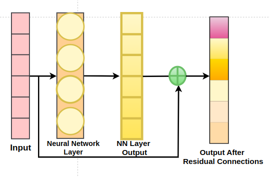
Residual connections play a vital role in addressing issues like vanishing and exploding gradients, contributing to the stability and efficiency of the training process. They act as a “shortcut” that allows gradients to flow freely through the network during backpropagation, thereby enhancing training ease and stability.

Implementation with Code

import torch
import torch.nn as nn

class ResidualBlock(nn.Module):
   def __init__(self, sublayer):
       super(ResidualBlock, self).__init__()
       self.sublayer = sublayer

   def forward(self, x):
       # Pass input through sublayer
       sublayer_output = self.sublayer(x)

       # Add residual connection
       output = x + sublayer_output
      return output

# Example usage
input_size = 512
output_size = 512  # Match the input size for the linear layer

# Define a simple sub-layer (e.g., linear transformation)
sublayer = nn.Linear(input_size, output_size)


# Create a residual block with the sub-layer
residual_block = ResidualBlock(sublayer)

# Generate a random input tensor
input_tensor = torch.randn(1, input_size)

# Forward pass through the residual block
output_tensor = residual_block(input_tensor)

# Print shapes for illustration
print("Input Shape:", input_tensor.shape)
print("Output Shape:", output_tensor.shape)

Layer Normalization

Layer normalization is crucial in stabilizing training within each sub-layer (such as attention and feed-forward layers) of a transformer block. Two common normalization techniques are batch normalization and layer normalization. Both methods transform activation values using a standard equation.

To obtain the normalized activation value, we subtract the mean and divide by the standard deviation of the original activation value. Batch normalization calculates a mean and standard deviation per dimension over the entire mini-batch, hence its name.

Layer normalization in a Decoder-Only transformer involves computing the mean and standard deviation over the input’s final dimension, eliminating dependency on the batch dimension and enhancing training stability by computing normalization statistics over the embedding dimension. Affine transformation is a common practice in deep neural networks, particularly with normalization layers. It involves normalizing the activation value using layer normalization and adjusting it further using a constant multiplier and additive constant, which are learnable parameters.

In a cake recipe, the normalization layer prepares the batter, while the affine transformation customizes the taste and texture. The constants γ and β act as the sugar and butter, making small adjustments to the normalized values to improve the neural network’s overall performance.

Layer normalization employs a modified standard deviation with a small constant (ε) in the denominator to prevent issues like dividing by zero and maintain stability.

Implementation with Code

import torch
import torch.nn as nn


class LayerNormalization(nn.Module):
   def __init__(self, features, eps=1e-6):
       super(LayerNormalization, self).__init__()
       self.gamma = nn.Parameter(torch.ones(features))
       self.beta = nn.Parameter(torch.zeros(features))
       self.eps = eps


   def forward(self, x):
       mean = x.mean(dim=-1, keepdim=True)
       std = x.std(dim=-1, keepdim=True)
       x_normalized = (x - mean) / (std + self.eps)
       output = self.gamma * x_normalized + self.beta
       return output


# Example usage
input_size = 512
batch_size = 10


# Create a layer normalization instance
layer_norm = LayerNormalization(input_size)


# Generate a random input tensor
input_tensor = torch.randn(batch_size, input_size)


# Forward pass through layer normalization
output_tensor = layer_norm(input_tensor)


# Print shapes and outputs for illustration
print("Input Shape:", input_tensor.shape)
print("Output Shape:", output_tensor.shape)
print("Output Mean:", output_tensor.mean().item())
print("Output Standard Deviation:", output_tensor.std().item())

Feed-Forward Transformation

In a decoder-only transformer block, there’s a step after the attention mechanism called the pointwise feed-forward transformation. This process involves passing each token vector through a small feed-forward neural network, which consists of two linear layers separated by an activation function.

When choosing an activation function for the feed-forward layers in a large language model , it’s important to consider performance. After comparing various activation functions, researchers found that the SwiGLU activation function delivers the best results given a fixed computational budget.
SwiGLU is widely favored and commonly used in popular large language models (LLMs) because of its effectiveness.

Constructing the Decoder-Only Transformer Model

We will now construct the decoder-only transformer model.

Step1: Model Inputs Construction

Token Embedding:

Token embeddings are essential in capturing the meaning of words or tokens within a decoder-only transformer model. Text undergoes tokenization, followed by conversion into high-dimensional embedding vectors through an embedding layer within the model.

The embedding layer functions like a table, assigning each token a unique integer index from the vocabulary. This index corresponds to a row in the embedding matrix, which has dimensions d columns and V rows (V is the size of our vocabulary). By looking up the token’s index in this matrix, we get its d-dimensional embedding.

During training, the model adjusts these embeddings based on the data it sees, allowing it to learn better representations of words over time. It’s like the model is learning to understand words better as it sees more examples, improving its performance.

Positional Embedding

Positional embeddings play a vital role in transformer models by providing essential information about the order of tokens in a sequence. Unlike recurrent or convolutional models, transformers lack inherent knowledge of token order, making positional embeddings necessary for understanding sequence structure.

One common method involves adding positional embeddings to each token in the input sequence. These embeddings have the same dimensionality as token embeddings (often denoted as d) and are trainable, meaning they adjust during training. Their purpose is to help the model differentiate tokens based on their positions in the sequence, enhancing the model’s ability to understand and process sequential data accurately.

Implementation with Code

import torch
import torch.nn as nn


class PositionalEncoding(nn.Module):
   def __init__(self, d_model, max_len=512):
       super(PositionalEncoding, self).__init__()
       self.d_model = d_model
       self.max_len = max_len

       # Create a positional encoding matrix
       pe = torch.zeros(max_len, d_model)
       position = torch.arange(0, max_len, dtype=torch.float32).unsqueeze(1)
       div_term = torch.exp(torch.arange(0, d_model, 2).float() * (-torch.log(torch.tensor(10000.0)) / d_model))
       pe[:, 0::2] = torch.sin(position * div_term)
       pe[:, 1::2] = torch.cos(position * div_term)
       pe = pe.unsqueeze(0)

       self.register_buffer('pe', pe)

   def forward(self, x)
       # Add positional embeddings to input token embeddings
       x = x + self.pe[:, :x.size(1)]

      return x

# Example usage
d_model = 512  # Dimensionality of token embeddings and positional embeddings
max_len = 100  # Maximum sequence length

# Create a positional encoding instance
positional_encoding = PositionalEncoding(d_model, max_len)

# Generate a random input token embedding tensor
input_token_embeddings = torch.randn(1, max_len, d_model)

# Forward pass through positional encoding
output_embeddings = positional_encoding(input_token_embeddings)

# Print shapes for illustration
print("Input Token Embeddings Shape:", input_token_embeddings.shape)
print("Output Token Embeddings Shape:", output_embeddings.shape)

Strategies for Positional Embeddings

There are two main strategies for generating positional embeddings:

• Learned Positional Embeddings: Positional embeddings, akin to token embeddings, can reside in an embedding layer and learn from data during training. This approach is straightforward to implement but may not generalize well to longer sequences than those seen during training.
• Fixed Positional Embeddings: These can also be created using mathematical functions like sine and cosine, as outlined in the text. These functions create embeddings based on the token’s absolute position in the sequence. While this approach is more generalizable, it requires defining a rule or equation for generating positional embeddings.

Overall, positional embeddings are essential for transformers to understand the sequential order of tokens, enabling them to process text and other sequential data effectively.

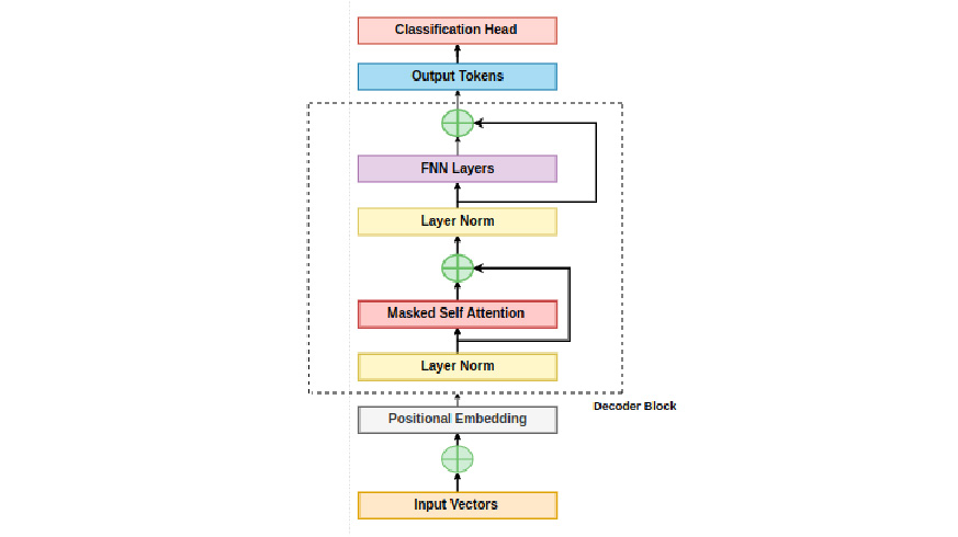
Step2: Model Body

The input sequence sequentially passes through multiple decoder-only transformer blocks.

In a decoder-only transformer model, after constructing the input by adding positional embeddings to token embeddings, it passes through a series of transformer blocks. The number of these blocks depends on the size of the model.

Model Architecture 

Increasing the model’s size can be achieved by either increasing the number of transformer blocks (layers) or by increasing the dimensionality (d) of token embeddings. Increasing d leads to larger weight matrices in attention and feed-forward layers. Typically, scaling up a decoder-only transformer model involves increasing both the number of layers and the hidden dimension.

Increasing the model’s parameters is achieved by increasing the number of attention heads within each attention layer. But this doesn’t directly affect the number of parameters if each attention head has a dimension of d.

Step3: Classification

A classification head predicts the next token in the sequence or performs text generation tasks. In the decoder-only transformer architecture, after passing the input sequence through the model’s body and obtaining a sequence of token vectors, we convert each token vector into a probability distribution over potential next tokens. This process involves adding an extra linear layer with input dimension d and output dimension V to the end of the model, creating a classification head.

Using this linear layer, we can generate a probability distribution for each token in the output sequence, enabling us to perform tasks such as:

• Next Token Prediction: This is the pretraining objective where the model learns to predict the next token for each token in the input sequence using a cross-entropy loss function.
• Inference: By sampling from the token distribution generated by the model, we can autoregressively determine the best next token, which is useful for text generation tasks.

The classification head enables text generation and predictions using learned token probabilities.

After processing our input through all decoder-only transformer blocks, we have two options. The first is to pass all output token embeddings through a linear classification layer, enabling us to apply a next token prediction loss across the entire sequence, typically done during pretraining. The second option involves passing only the final output token through the linear classification layer. Allowing for the sampling of the next token during inference.

Implementation with Code

import torch
import torch.nn as nn

class ClassificationHead(nn.Module):
   def __init__(self, input_size, vocab_size):
       super(ClassificationHead, self).__init__()
       self.linear = nn.Linear(input_size, vocab_size)

   def forward(self, x):
       # Pass token embeddings through linear layer
       output_logits = self.linear(x)
       return output_logits

# Example usage
input_size = 512
vocab_size = 10000  # Example vocabulary size

# Create a classification head instance
classification_head = ClassificationHead(input_size, vocab_size)

# Generate a random input token embedding tensor
input_token_embeddings = torch.randn(10, input_size)  # Batch size of 10

# Forward pass through classification head
output_logits = classification_head(input_token_embeddings)

# Print shapes for illustration
print("Input Token Embeddings Shape:", input_token_embeddings.shape)
print("Output Logits Shape:", output_logits.shape)

Conclusion

The Decoder-Only Transformer architecture excels in generating sequential data, particularly in natural language tasks. Its key components, including token embeddings, positional embeddings, normalization techniques, and the classification head, work together to capture semantics, understand token order, ensure training stability, and enable tasks like text generation. With its versatility and effectiveness, the Decoder-Only Transformer stands as a powerful tool in natural language processing applications.

Key Takeaways

• The Decoder-Only Transformer, a variant of the Transformer model, performs tasks like language translation and text generation.
•  Components such as attention mechanisms, positional embeddings, normalization techniques, feed-forward transformations, and residual connections are crucial for the model’s effectiveness.
• Token embeddings map tokens to high-dimensional spaces, capturing semantic information.
•  Positional embeddings provide positional information to understand token order in sequences.
• Layer normalization and affine transformations contribute to training stability and performance.
•  The classification head enables tasks like next token prediction and text generation.
• Investigate token embeddings and their significance in capturing semantic information in the model.
• Examine the classification head’s role in next token prediction and text generation in the Decoder-Only Transformer.

Frequently Asked Questions