Comprehensive Guide on Linear Discriminant Analysis

Introduction

Linear Discriminant Analysis (LDA) is a supervised technique used for maximizing class separability. The LDA dimensional reduction technique aims to enhance computational efficiency and mitigate overfitting caused by the curse of dimensionality in non-regularized models like Decision Trees. Linear Discriminant Analysis (LDA) seeks to identify the feature subspace that maximizes the separation between classes. In this article we’ll understand how LDA is used for dimensionality reduction and classification tasks.

Learning objectives

• Understand the theoretical foundations of Linear Discriminant Analysis (LDA) and its assumptions.
• Learn how LDA is applied for dimensionality reduction to reduce the number of features while preserving class discriminatory information.
• Understand the differences between LDA and PCA and know when to use them.
• Explore the process of using LDA for classification tasks.
• Gain insights into the differences between LDA and Quadratic Discriminant Analysis (QDA) for classification.
• Learn about the implementation of LDA using python. 

LDA for Dimensionality Reduction

Linear Discriminant Analysis (LDA) is utilized in supervised learning scenarios where labeled data is available for training. LDA also operates as a dimensionality reduction technique, similar to Principal Component Analysis (PCA). Its objective lies in deriving a linear combination of features that optimally separates these classes. 

In LDA, the no. of linear discriminants is at most c -1 , here c is the number of class labels. This is because the in-between scatter matrix SB is the sum of c matrices with rank 1 or less, so there can be at most c-1 eigenvalues.

LDA seeks the directions (eigenvectors) that maximize the ratio of the determinant of the between-class scatter matrix to the within-class scatter matrix. These eigenvectors are also referred to as discriminant vectors, and they define the directions along which the data should be projected to achieve maximum class separation.

One of the foundational assumptions underlying LDA is the Gaussian distribution of features within each class, alongside the assumption of equal covariance matrices across different classes. These assumptions are pivotal for LDA’s effectiveness in discerning class boundaries and making accurate classifications. The optimization objective of LDA revolves around maximizing between-class scatter while simultaneously minimizing within-class scatter. This optimization process involves determining the projection that maximizes the ratio of between-class scatter to within-class scatter, thereby refining the discriminative capabilities of the model.

Upon completion of the training phase, Linear Dimensionality Analysis generates a decision boundary that best delineates different classes within the dataset. Typically as a hyperplane in the feature space, this decision boundary plays a crucial role in facilitating classification tasks by delineating the boundaries between different classes.

Steps in LDA Dimensionality Reduction

• Standardize the d-dimensional dataset (d is the number of features) using z-score normalization. 
  • x′ is the standardized or normalized value of x
  • x is the original value of the variable
  • μ is the mean (average) value of the variable x
  • σ is the standard deviation of the variable 

• For each class we have to compute the d-dimensional mean vector. Each mean vector μ stores the mean feature value for each sample of class i. LDA is a supervised technique as it is using class-wise information here.

• Construct the within-class scatter matrix Sw and between-class scatter matrix Sb.

The Scatter matrix is used to make an estimation about the covariance matrix. There exist two types of scatter matrices:

• Between-class scatter (Sb): The between-class scatter (Sb) matrix represents the degree of scatter between classes as a covariance matrix of means of all classes.
• Within-class scatter (Sw): The (Sw) matrix assesses the spread around the means of individual classes.

The assumption that we are making when we are computing the scatter matrices is that the class labels in the training set are uniformly distributed.

First we calculate the individual scatter matrices Si of each individual class i using the mean: 

Now, summing up the individual scatter matrices gives the the within-class scatter matrix SW: 

The between-class scatter matrix SB can be calculated using : 

m is the overall mean that is computed, including samples from all classes.

Compute the eigenvalues and corresponding eigenvectors of the matrix inv(Sw)*(Sb).

• Eigenvalues: Eigenvalues represent the amount of variance explained by the corresponding eigenvectors. In LDA, eigenvalues indicate the importance of the corresponding discriminant vectors. Larger eigenvalues imply greater separation between classes along the corresponding eigenvectors.
• Eigenvectors: Eigenvectors in LDA represent the directions along which the data should be projected to achieve maximum class separation. These eigenvectors are computed from the scatter matrices and correspond to the directions of maximum between-class scatter relative to within-class scatter.

• Arrange the eigenvalues in descending order to prioritize the corresponding eigenvectors.

• Select N eigenvectors corresponding to the N largest eigenvalues to establish the d x k-dimensional transformation matrix W; these eigenvectors constitute the columns of the matrix.

• Use the transformation matrix W to project the samples onto the new feature subspace,

using the transformation matrix W that we can now transform the training dataset by multiplying the matrices: X′= XW

LDA vs PCA for Dimensionality Reduction

While both PCA and LDA are linear transformation techniques that are used to reduce the number of dimensions in the data. 

PCA attempts to find the orthogonal component axes of maximum variance in a dataset and it doesn’t take into account class labels or any information about the classes. LDA find’s the feature subspace that optimizes class separability while minimizing the variance within each class.

It is also worth mentioning that PCA happens to be an unsupervised algorithm, whereas LDA is a supervised algorithm.

PCA does not make any assumptions about the distribution of the data. In Linear Dimensionality Analysis an assumption is that the data is normally distributed within each class. Meaning each class has its own multivariate normal distribution.

In Linear Discriminant Analysis (LDA), the number of linear discriminants is at most c−1, where c is the number of class labels. This means that if there are c classes in the data, LDA can generate at most c−1 linear discriminants. In Principal Component Analysis (PCA), the number of principal components is equal to the number of original features in the dataset, or the rank of the covariance matrix of the data. This means that PCA can potentially produce as many principal components as there are original features in the dataset.

Python code to analyze dimensionality reduction using PCA and LDA

import numpy as np
import matplotlib.pyplot as plt
from sklearn.datasets import make_classification
from sklearn.decomposition import PCA
import pandas as pd
# Generating the dataset

x, y = make_classification(n_samples=250, n_features=20, n_classes=2, random_state=92)
data = pd.DataFrame(x)
data.head()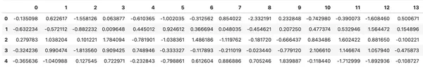

# Applying PCA
pca = PCA(n_components=1)
x_pca = pca.fit_transform(x)

# Applying LDA
lda = LinearDiscriminantAnalysis(n_components=1)
x_lda = lda.fit_transform(x, y)

# Plotting results
plt.figure(figsize=(12, 6))
# Plotting PCA
plt.subplot(1, 2, 1)
plt.title("PCA")
plt.scatter(x_pca, np.zeros_like(x_pca), c=y, cmap='coolwarm')
plt.xlabel('Principal Component 1')

# Plotting LDA
plt.subplot(1, 2, 2)
plt.title("LDA")
plt.scatter(x_lda, np.zeros_like(x_lda), c=y, cmap='coolwarm')
plt.xlabel('LDA Component 1')
plt.tight_layout()
plt.show()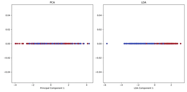

from sklearn.linear_model import LogisticRegression
from sklearn.model_selection import train_test_split as tts
from sklearn.metrics import accuracy_score
lr=LogisticRegression()
x_train, x_test, y_train, y_test=tts(x_pca,y,stratify=y,random_state=92)
lr.fit(x_train, y_train)
predictions=lr.predict(x_test)
print('Logistic regression on Prinicipal components gives an accuracy: ',
accuracy_score(predictions,y_test))

x_train, x_test, y_train, y_test=tts(x_lda,y,stratify=y,random_state=92)
lr.fit(x_train, y_train)
predictions=lr.predict(x_test)
print('Logistic regression on Linear Discriminants gives an accuracy: ',
      accuracy_score(predictions,y_test))

As you can see LDA captures the class-discriminatory information as it considers the separation between classes when projecting the data onto a lower-dimensional space. It aims to maximize the between-class variance while minimizing the within-class variance. In contrast, PCA only considers the overall variance in the data, which may not necessarily optimize class separability. The Logistic Regression model is clearly performing poorly on the dimensionality reduced data by PCA.

When to use LDA?

Linear Discriminant Analysis (LDA) is used for supervised dimensionality reduction tasks, particularly when the target variables are categorical and there is a clear distinction between classes.

Linear Discriminant Analysis (LDA) serves multiple purposes, including dimensionality reduction, classification, and visualization of high-dimensional data.

LDA to visualize high dimensional data:

import numpy as np
import pandas as pd
import plotly.express as px
from sklearn.datasets import fetch_openml
from sklearn.discriminant_analysis import LinearDiscriminantAnalysis as LDA
import warnings
warnings.filterwarnings('ignore')

# Load MNIST dataset
mnist = fetch_openml('mnist_784', version=1)
X = mnist.data
y = mnist.target.astype(int)

# Create LDA instance and fit the data
lda = LDA(n_components=2)
X_lda = lda.fit_transform(X, y)

# Create a DataFrame for Plotly
data = {
   'LD1': X_lda[:, 0],
   'LD2': X_lda[:, 1],
   'label': y
}

df = pd.DataFrame(data)
# Plot using Plotly
fig = px.scatter(df, x='LD1', y='LD2', color='label', title='MNIST Dataset Visualization using LDA')
# Set aspect ratio to make the plot more square
fig.update_layout(
   autosize=False,
   width=800,
   height=600,
   margin=dict(l=0, r=0, b=0, t=30),
)
fig.show()

Using Linear Discriminant Analysis (LDA) Dimensionality Reduction to shrink the number of features from 784 to 2 Linear Discriminants helped us visualize the MNIST dataset. This dataset includes images of handwritten numbers from 0 to 9, with the target variable represented using 10 labels from 0 to 9. Each number is visualized using a different color, ranging from blue to yellow.

When to use PCA?

Principal Component Analysis (PCA) is the preferred choice for unsupervised dimensionality reduction tasks, particularly when dealing with continuous target variables or when there’s no clear distinction between classes.

PCA excels in denoising images by capturing the most significant features and reconstructing the image without the noise present in the original data.

Additionally, Kernel PCA (KPCA) offers a solution for transforming non-linearly separable data onto a new, lower-dimensional subspace where the data becomes linearly separable. This technique is valuable when traditional PCA fails to capture complex relationships within the data.

Classification using LDA

The probabilistic interpretation of Linear Discriminant Analysis (LDA) provides a framework for understanding how the model makes classifications based on the statistical properties of the data. In this interpretation, LDA assumes that the features within each class follow a Gaussian (normal) distribution. By modeling these distributions, LDA can probabilistically assign new data points to different classes.

The Gaussian Distribution Assumption:

LDA assumes that the features within each class follow a multivariate Gaussian distribution.

The mathematical formula for the probability density function (PDF) of a multivariate Gaussian distribution is:

Given a new data point x, Linear Discriminant Analysis (LDA) computes the posterior probability of each class given the observed features.

Using Bayes’ theorem, we can compute the posterior probability:

LDA predicts by assessing the likelihood that a new input set aligns with each class. The output class is identified as the class resulting in the greatest likelihood.

From Bayes Theorem, the model computes these probabilities. Bayes Theorem estimates the likelihood of the output class (k) for a specific input (x), leveraging the probabilities associated with each class and the likelihood of the data belonging to each class.

Where P(x/y=k) refers to the base probability of each class (k) observed in your training data. In Bayes’ Theorem, this is known as the prior probability.

The Gaussian distribution function calculates P(y=k), which is the estimated probability of x belonging to class k.

LDA vs QDA for Classification

LDA is particularly suitable for tasks involving linearly separable classes. Quadratic Discriminant Analysis (QDA) becomes more appropriate when classes exhibit separation by quadratic boundaries.

The QDA classifier uses the log of the posterior probability:

where the constant term Cst corresponds to the denominator P(x), in addition to other constant terms from the Gaussian. The predicted class is the one that maximizes this log-posterior.

Whereas LDA is a special case of QDA:

Here, we assume that the Gaussians for each class share the same covariance matrix.

 k = for all k.

Note: The covariance matrix k is a normalized version of the Within-class scatter matrix (Sw). 

This changes the log posterior to:

The term is the Mahalanobis Distance between the sample x and the mean k. This Mahalanobis distance tells how close or far x is from k, while also accounting for the variance of each of the features. We can thus interpret LDA as assigning x to the class whose has the closest Mahalanobis distance, while also considering the class prior probabilities.

From all the formulas, we can say that LDA has a linear decision surface. Whereas, QDA has no assumptions on the covariance matrices k of the Gaussians, which leads to a quadratic decision surface.

Python code to implement LDA for classification

import matplotlib.pyplot as plt
import numpy as np
from sklearn.datasets import make_classification
from sklearn.discriminant_analysis import LinearDiscriminantAnalysis


# Generate linearly separable data
X, y = make_classification(n_samples=100, n_features=2, n_classes=2, n_clusters_per_class=1, n_redundant=0, n_informative=2, class_sep=2, random_state=42)


# Fit LDA classifier
clf = LinearDiscriminantAnalysis()
clf.fit(X, y)


# Plot decision boundary
x_min, x_max = X[:, 0].min() - 1, X[:, 0].max() + 1
y_min, y_max = X[:, 1].min() - 1, X[:, 1].max() + 1
xx, yy = np.meshgrid(np.arange(x_min, x_max, 0.1),
                    np.arange(y_min, y_max, 0.1))
Z = clf.predict(np.c_[xx.ravel(), yy.ravel()])
Z = Z.reshape(xx.shape)


plt.contourf(xx, yy, Z, alpha=0.4)
plt.scatter(X[:, 0], X[:, 1], c=y, s=20, edgecolor='k')
plt.title('LDA for classification')
plt.xlabel('Feature 1')
plt.ylabel('Feature 2')
plt.show()

We can say that LDA is well-suited for linearly separable data as it assumes the data can be separated by a linear decision boundary. We can also see that LDA seeks to find the decision boundary that maximizes the separation between classes.

Python code to implement QDA to separate concentric circles

from sklearn.datasets import make_circles
from sklearn.model_selection import train_test_split
from sklearn.discriminant_analysis import QuadraticDiscriminantAnalysis
from sklearn.discriminant_analysis import LinearDiscriminantAnalysis
from sklearn.metrics import accuracy_score
import numpy as np
import matplotlib.pyplot as plt


# Generating the data
X, y = make_circles(n_samples=1000, random_state=123, noise=0.1, factor=0.2)
# Plotting the data points
plt.scatter(X[y == 0, 0], X[y == 0, 1], color='purple', marker='o', alpha=0.5)
plt.scatter(X[y == 1, 0], X[y == 1, 1], color='gold', marker='o', alpha=0.5)


# Displaying the plot
plt.show()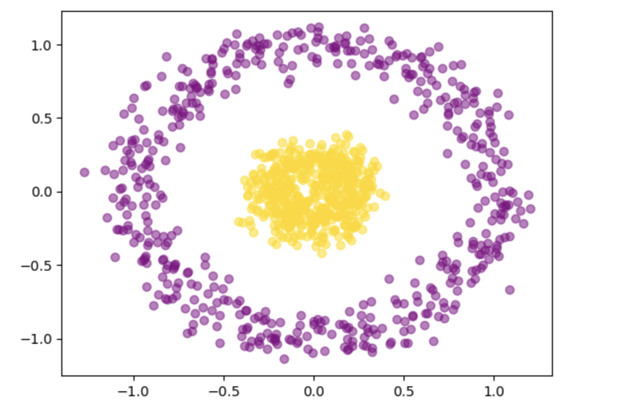

# Splitting the data into training and testing sets
X_train, X_test, y_train, y_test = train_test_split(X, y, test_size=0.3, random_state=42)


# Initializing and fitting the QDA model
qda = QuadraticDiscriminantAnalysis()
qda.fit(X_train, y_train)


# Define a meshgrid that covers the range of the data
x_min, x_max = X[:, 0].min() - 0.1, X[:, 0].max() + 0.1
y_min, y_max = X[:, 1].min() - 0.1, X[:, 1].max() + 0.1
xx, yy = np.meshgrid(np.arange(x_min, x_max, 0.01),
                    np.arange(y_min, y_max, 0.01))


# Predict the class labels for each point on the meshgrid
Z = qda.predict(np.c_[xx.ravel(), yy.ravel()])
Z = Z.reshape(xx.shape)


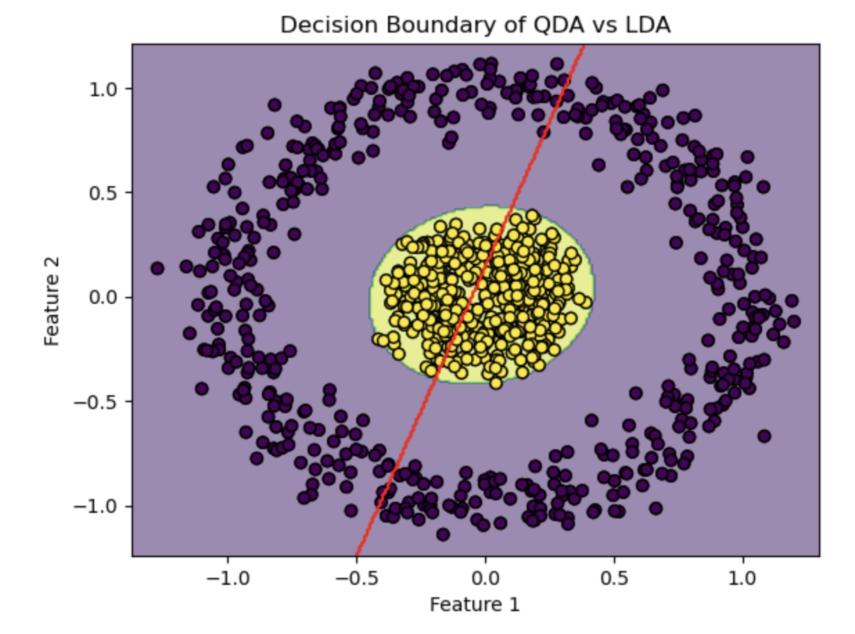
# Plotting the decision boundary along with the training data points
plt.contourf(xx, yy, Z, alpha=0.3)
plt.scatter(X[:, 0], X[:, 1], c=y, marker='o', edgecolors='k')
plt.xlabel('Feature 1')
plt.ylabel('Feature 2')


# Initialize and fit the LDA model
lda = LinearDiscriminantAnalysis()
lda.fit(X_train, y_train)


# Predict the class labels for each point on the meshgrid using LDA
Z_lda = lda.predict(np.c_[xx.ravel(), yy.ravel()])
Z_lda = Z_lda.reshape(xx.shape)


# Plotting the decision boundaries along with the training data points
plt.contourf(xx, yy, Z, alpha=0.3, cmap='viridis')
plt.contour(xx, yy, Z_lda, levels=[0.5], colors='red')  # LDA decision boundary
plt.scatter(X[:, 0], X[:, 1], c=y, marker='o', edgecolors='k')
plt.xlabel('Feature 1')
plt.ylabel('Feature 2')
plt.title('Decision Boundary of QDA vs LDA')


plt.show()

# Predicting the labels for the testing data
y_pred1 = qda.predict(X_test)


# Calculating the accuracy of the model
accuracy = accuracy_score(y_test, y_pred1)
print("Accuracy of QDA classifier:", accuracy)


y_pred2 = lda.predict(X_test)


# Calculating the accuracy of the model
accuracy = accuracy_score(y_test, y_pred2)
print("Accuracy of LDA classifier:", accuracy)

Quadratic Discriminant Analysis (QDA) separates concentric circles effectively, demonstrating its versatility in handling complex data. However, LDA struggles with low accuracy in this case.

Conclusion

Linear Discriminant Analysis (LDA) presents a distinct approach to dimensionality reduction compared to standard Principal Component Analysis (PCA). While PCA emphasizes maximizing variance along orthogonal axes, LDA, in contrast to PCA, is a technique for supervised dimensionality reduction, it considers class information in the training dataset to attempt to maximize the class-separability in a linear feature space. In case of non-linear feature space a nonlinear feature extractor, kernel PCA (KPCA) that employs the kernel trick and a temporary projection into a higher-dimensional feature space, this lets you to compress datasets consisting of nonlinear features onto a lower-dimensional subspace where the classes became linearly separable. 

Linear Discriminant Analysis (LDA) classifier stands as a useful tool for supervised learning and classification tasks as well. You can employ a Quadratic Discriminant Analysis (QDA) classifier when the feature space separates by a quadratic boundary. It’s worth mentioning that Applications of Linear Discriminant Analysis (LDA) extend to document classification, where it aids in categorizing documents based on their content and pattern recognition tasks, where it helps discern patterns or features in data.