Geospatial Data Analysis with Geemap
A Python library for creating interactive maps with Google Earth Engine and ipyleaflet.
Illustration by Author
Geospatial data analysis is a field addressed to deal with, visualize and analyze a special type of data, called geospatial data. Compared to the normal data, we have tabular data with an additional column, the location information, such as latitude and longitude.
There are two main types of data: vector data and raster data. When dealing with vector data, you still have a tabular dataset, while raster data are more similar to images, such as satellite images and aerial photographs.
In this article, I am going to focus on raster data provided by Google Earth Engine, a cloud computing platform that provides a huge data catalog of satellite imagery. This kind of data can be easily mastered from your Jupyter Notebook using a life-saving Python package, called Geemap. Let’s get started!
What is Google Earth Engine?
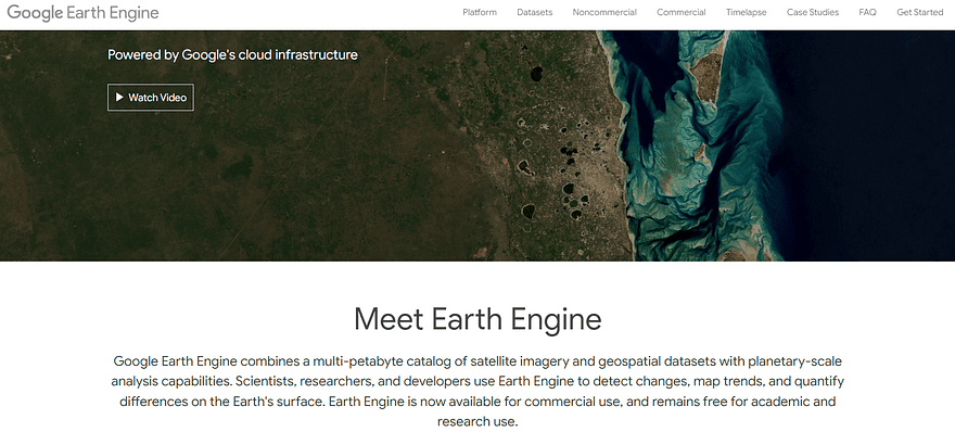
Screenshot by Author. Home page of Google Earth Engine.
Before getting started with the Python Library, we need to understand the potential of Google Earth Engine. This cloud-based platform, powered by Google Cloud platform, hosts public and free geospatial datasets for academic, non-profit and business purposes.
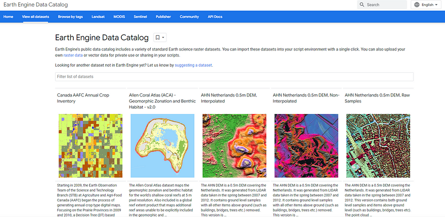
Screenshot by Author. Overview of Earth Engine Data Catalog.
The beauty of this platform is that it provides a multi-petabyte catalog of raster and vector data, stored on the Earth Engine servers. You can have a fast overview from this link. Moreover, it provides APIs to facilitate the analysis of raster datasets.
What is Geemap?
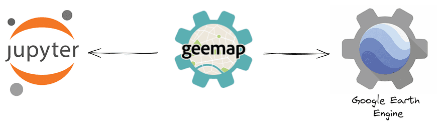
Illustration by Author. Geemap library.
Geemap is a Python library that allows to analyze and visualize huge amounts of geospatial data from Google Earth Engine.
Before this package, it was already possible to make computational requests through JavaScript and Python APIs, but Python APIs had limited functionalities and lacked documentation.
To fill this gap, Geemap was created to permit users to access resources of Google Earth Engine with few lines of code. Geemap is built upon eartengine-api, ipyleaflet and folium.
To install the library, you just need the following command:
pip install geemap
I recommend you experiment with this amazing package in Google Colab to understand its full potential. Take a look at this free book written by professor Dr. Qiusheng Wu for getting started with Geemap and Google Earth Engine.
How to Access Earth Engine?
First, we need to import two Python libraries, that will be used within the tutorial:
import ee
import geemap
In addition to geemap, we have imported the Earth Engine Python client library, called ee.
This Python library can be utilized for the authentication on Earth Engine, but it can be faster by using directly the Geemap library:
m = geemap.Map()
m
You need to click the URL returned by this line of code, which will generate the authorization code. First, select the cloud project and, then, click the “GENERATE TOKEN” button.
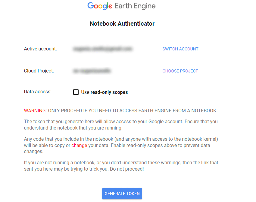
Screenshot by Author. Notebook Authenticator.
After, it will ask you to choose the account. I recommend taking the same account of Google Colab if you are using it.
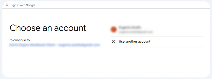
Screenshot by Author. Choose an account.
Then, click the check box next to Select All and press the “Continue” button. In a nutshell, this step allows the Notebook Client to access the Earth Engine account.
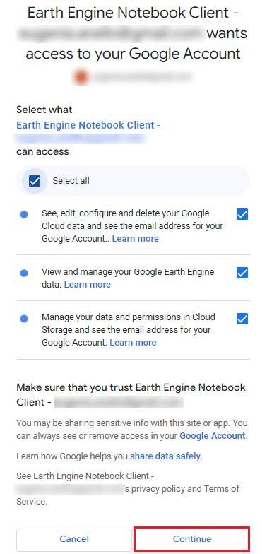
Screenshot by Author. Allow the Notebook Client to access your Earth Engine account.
After this action, the authentication code is generated and you can paste it into the notebook cell.
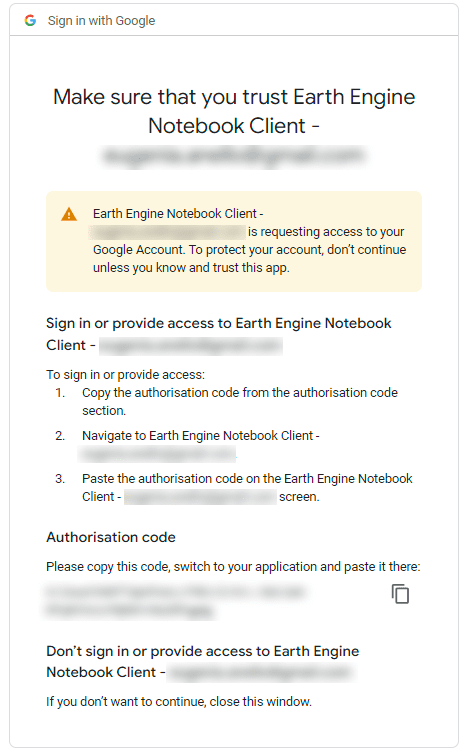
Screenshot by Author. Copy the Authentication Code.
Once the verification code is entered, you can finally create and visualize this interactive map:
m = geemap.Map()
m
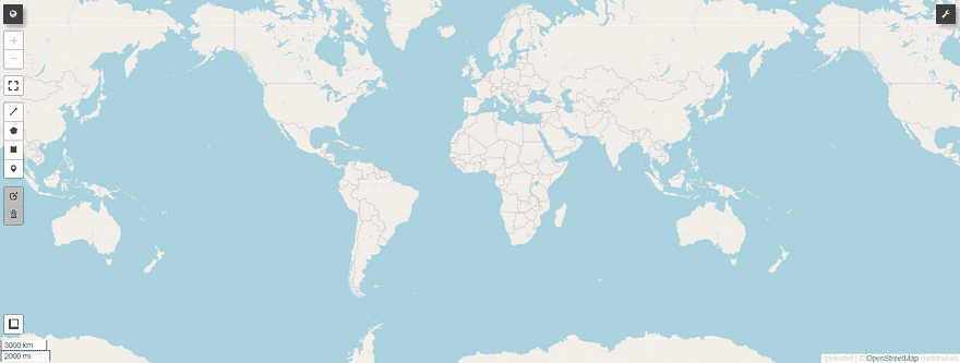
For now, you are just observing the base map on top of ipyleaflet, a Python package that enables the visualization of interactive maps within the Jupyter Notebook.
Create Interactive Maps
Previously, we have seen how to authenticate and visualize an interactive map using a single line of code. Now, we can customize the default map by specifying the latitude and longitude of the centroid, the level of zoom and the height. I have chosen the coordinates of Rome for the centre to focus on the map of Europe.
m = geemap.Map(center=[41, 12], zoom=6, height=600)
m
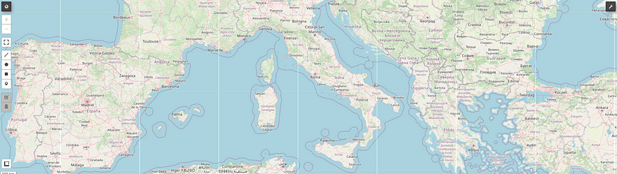
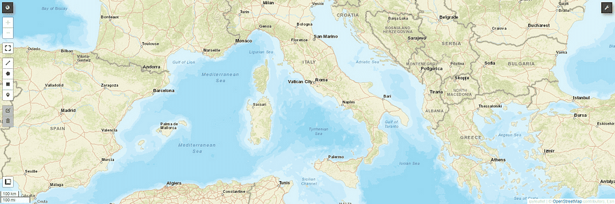
If we want to change the base map, there are two possible ways. The first way consists of writing and running the following code line:
m.add_basemap("ROADMAP")
m
Alternatively, you can change manually the base map by clicking the icon of ring spanner positioned at the right.
Moreover, we see the list of base maps provided by Geemap:
basemaps = geemap.basemaps.keys()
for bm in basemaps:
   print(bm)
This is the output:
OpenStreetMap
Esri.WorldStreetMap
Esri.WorldImagery
Esri.WorldTopoMap
FWS NWI Wetlands
FWS NWI Wetlands Raster
NLCD 2021 CONUS Land Cover
NLCD 2019 CONUS Land Cover
...
As you can notice, there is a long series of base maps, most of them available thanks to OpenStreetMap, ESRI and USGS.
Earth Engine Data Types
Before showing the full potential of Geemap, it’s important to know two main data types in Earth Engine. Take a look at the Google Earth Engine’s documentation for more details.
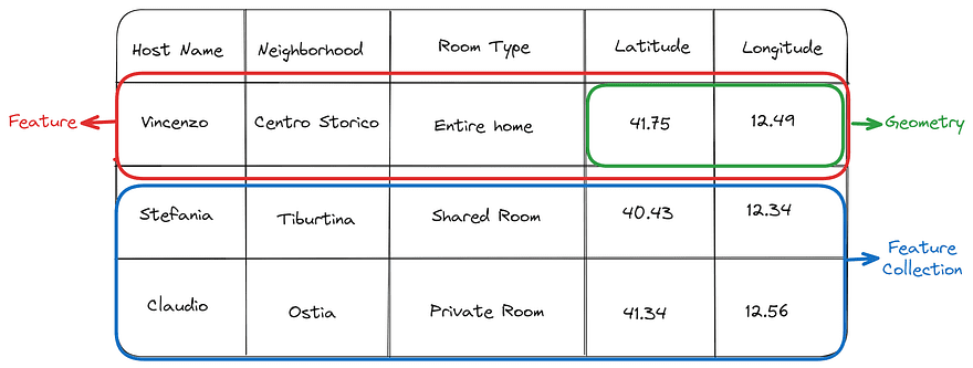
Illustration by Author. Example of vector data types: Geometry, Feature and FeatureCollection.
When handling vector data, we use principally three data types:
- Geometry stores the coordinates needed to draw the vector data on a map. Three main types of geometries are supported by Earth Engine: Point, LineString and Polygon.
- Feature is essentially a row that combines geometry and non-geographical attributes. It’s very similar to the GeoSeries class of GeoPandas.
- FeatureCollection is a tabular data structure that contains a set of features. FeatureCollection and GeoDataFrame are almost identical conceptually.
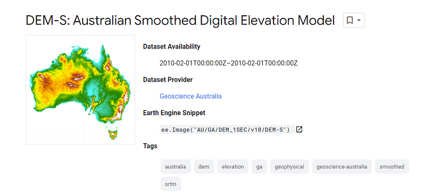
Screenshot by Author. Example of Image data type. It shows the Australian Smoothed Digital Elevation Model (DEM-S)
In the world of raster data, we focus on Image objects. Google Earth Engine’s Images are composed of one or more brands, where each band has a specific name, estimated minimum and maximum, and description.
If we have a collection or time series of images, ImageCollection is more appropriate as a data type.
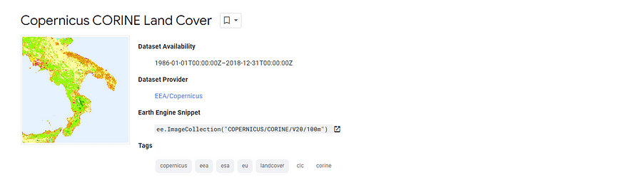
Screenshot by Author. Copernicus CORINE Land Cover.
We visualize the satellite imagery showing the land cover map of Europe. This dataset provides the changes between 1986 and 2018.
First, we load the image using ee.Image and, then, select the band “landcover”. Finally, let’s visualize the image by adding the loaded dataset to the map as a layer using Map.addLayer.
Map = geemap.Map()
dataset = ee.Image('COPERNICUS/CORINE/V20/100m/2012')
landCover = dataset.select('landcover')
Map.setCenter(16.436, 39.825, 6)
Map.addLayer(landCover, {}, 'Land Cover')
Map
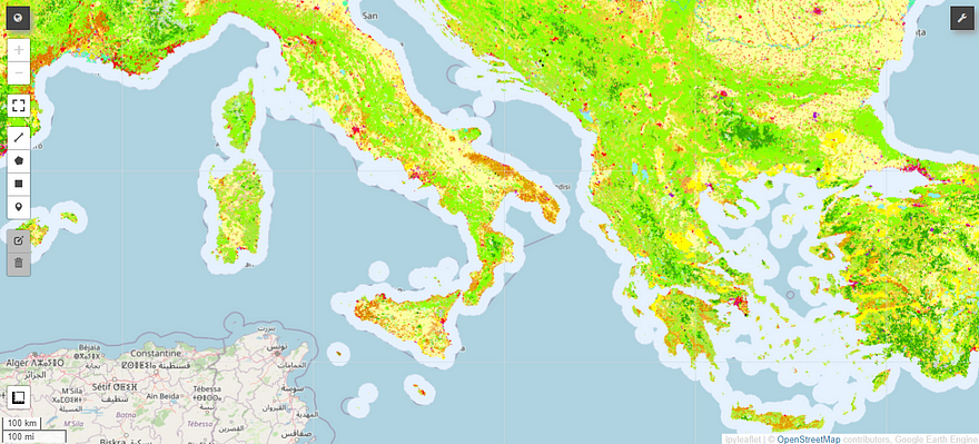
Screenshot by Author.
Similarly, we can do the same thing to load and visualize the satellite imagery showing the land cover map of Europe. This dataset provides the changes between 1986 and 2018.
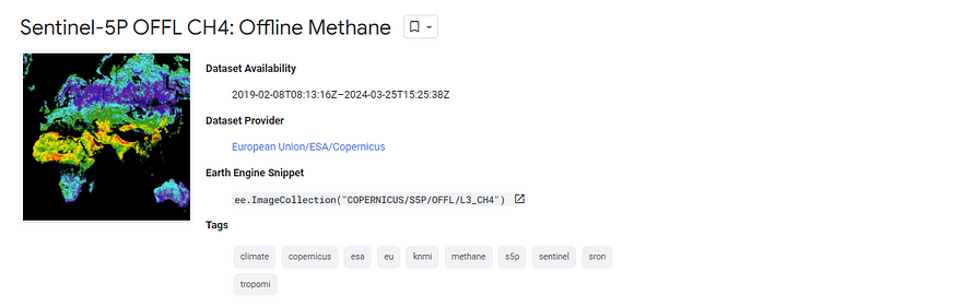
Screenshot by Author. Offline high-resolution imagery of methane concentrations.
To visualize an Earth Engine ImageCollection, the lines of code are similar, except for ee.ImageCollection.
Map = geemap.Map()
collection = ee.ImageCollection('COPERNICUS/S5P/OFFL/L3_CH4').select('CH4_column_volume_mixing_ratio_dry_air').filterDate('2019-06-01', '2019-07-16')
band_viz = {
 'min': 1750,
 'max': 1900,
 'palette': ['black', 'blue', 'purple', 'cyan', 'green', 'yellow', 'red']
}

Map.addLayer(collection.mean(), band_viz, 'S5P CH4')
Map.setCenter(0.0, 0.0, 2)
Map
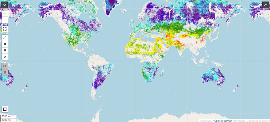
Screenshot by Author.
That’s great! From this map, we notice how Methane, one of the most important contributors to the greenhouse effect, is distributed within the globe.
Final Thoughts
This was an introductory guide that can help you work with Google Earth Engine data using Python. Geemap is the most complete Python library to visualize and analyze this type of data.
If you want to go deeper into this package, you can take a look at the resources I suggested below.
The code can be found here. I hope you found the article useful. Have a nice day!
Useful resources:
- Google Earth Engine
- Geemap Documentation
- Book Earth Engine and Geemap: Geospatial Data Science with Python
Eugenia Anello is currently a research fellow at the Department of Information Engineering of the University of Padova, Italy. Her research project is focused on Continual Learning combined with Anomaly Detection.