Regularization in Machine Learning

Introduction

When training a machine learning model, the model can be easily overfitted or under fitted. To avoid this, we use regularization in machine learning to properly fit the model to our test set. Regularization techniques help reduce the possibility of overfitting and help us obtain an optimal model. In this article titled ‘The Ultimate Guide to Regularization in Machine Learning, you will learn everything you need to know about regularization ML.

Learning Objectives:

• Understand the concept of regularization in machine learning and its role in preventing overfitting and underfitting.
• Learn about the different regularization techniques, such as Ridge, Lasso, and Elastic Net regularization.
• Gain practical knowledge of implementing regularization techniques using Python and scikit-learn.

This article was published as a part of the Data Science Blogathon.

What is Regularization in Machine Learning

Regularization is a technique used in machine learning to prevent overfitting and improve the generalization performance of models. In essence, regularization adds a penalty term to the loss function, discouraging the model from learning overly complex patterns that may not generalize well to unseen data. This helps create simpler, more robust models.

The main benefits of regularization include:

• Reducing overfitting: By constraining the model’s complexity, regularization helps prevent the model from memorizing noise or irrelevant patterns in the training data.
• Improving generalization: Regularized models tend to perform better on new, unseen data because they focus on capturing the underlying patterns rather than fitting the training data perfectly.
• Enhancing model stability: Regularization makes models less sensitive to small fluctuations in the training data, leading to more stable and reliable predictions.
• Enabling feature selection: Some regularization techniques, such as L1 regularization, can automatically identify and discard irrelevant features, resulting in more interpretable models.

The most common regularization techniques are L1 regularization (Lasso), which adds the absolute values of the model weights to the loss function, and L2 regularization (Ridge), which adds the squared values of the weights. By incorporating these penalty terms, regularization strikes a balance between fitting the training data and keeping the model simple, ultimately leading to better performance on new data.

Also Read: Complete Guide to Regularization Techniques in Machine Learning

Understanding Overfitting and Underfitting

To train our machine learning model, we provide it with data to learn from. The process of plotting a series of data points and drawing a line of best fit to understand the relationship between variables is called Data Fitting. Our model is best suited when it can find all the necessary patterns in our data and avoid random data points, and unnecessary patterns called noise.

If we allow our machine learning model to look at the data too many times, it will find many patterns in our data, including some that are unnecessary. It will learn well on the test dataset and fits very well. It will learn important patterns, but it will also learn from the noise in our data and will not be able to make predictions on other data sets.

A scenario where a machine learning model tries to learn from the details along with the noise in the data and tries to fit each data point to a curve is called Overfitting.

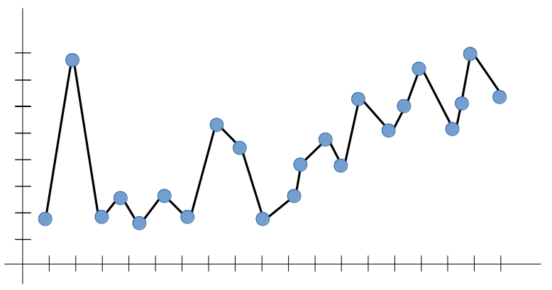
In the figure below, we can see that the model is fit for every point in our data. If new data is provided, the model curves may not match the patterns in the new data, and the model may not predict very well.

Conversely, when we haven’t allowed the model to look at our data enough times, it won’t be able to find patterns in our test data set. It won’t fit our test data set properly and won’t work on new data either.

Underfitting occurs when a machine learning model fails to learn the relationship between variables in the test data or to predict or classify a new data point.

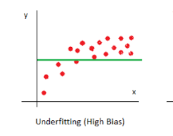
The image below shows an underequipped model. We can see that it doesn’t fit the data given correctly. He did not find patterns in the data and ignored much of the data set. It cannot work with both known and unknown data.

What are the Bias and Variance?

Bias comes out when the algorithm has limited flexibility to learn from the dataset. These models pay little attention to the training data and oversimplify the model, so the validation or prediction errors and training errors follow similar trends. Such models always lead to high errors in the training and test data. High bias causes under-adjustment in our model.

The variance defines the sensitivity of the algorithm to specific data sets. A high-variance model pays close attention to the training data and does not generalize, so the validation or prediction errors are far from each other. Such models usually perform very well on the training data but have a high error rate on the test data. High deviation causes an overshoot in our model.

An optimal model is one in which the model is sensitive to the pattern in our model but can also generalize to new data. This occurs when both bias and variance are optimal. We call this the Bias-Variance Tradeoff, and we can achieve this in models over or under-fitted models using regression.

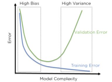
The above figure shows that when the bias is high, the error in both the test and training sets is also high. When the deviation is high, the model performs well on our training set and gives a low error, but the error on our test set is very high. In the middle of this, there is a region where bias and variance are in perfect balance with each other here too, but training and testing errors are low.

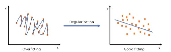
Regularization in Machine Learning?

It refers to techniques used to calibrate machine learning models to minimize the adjusted loss function and avoid overfitting or underfitting.

Regularization Techniques

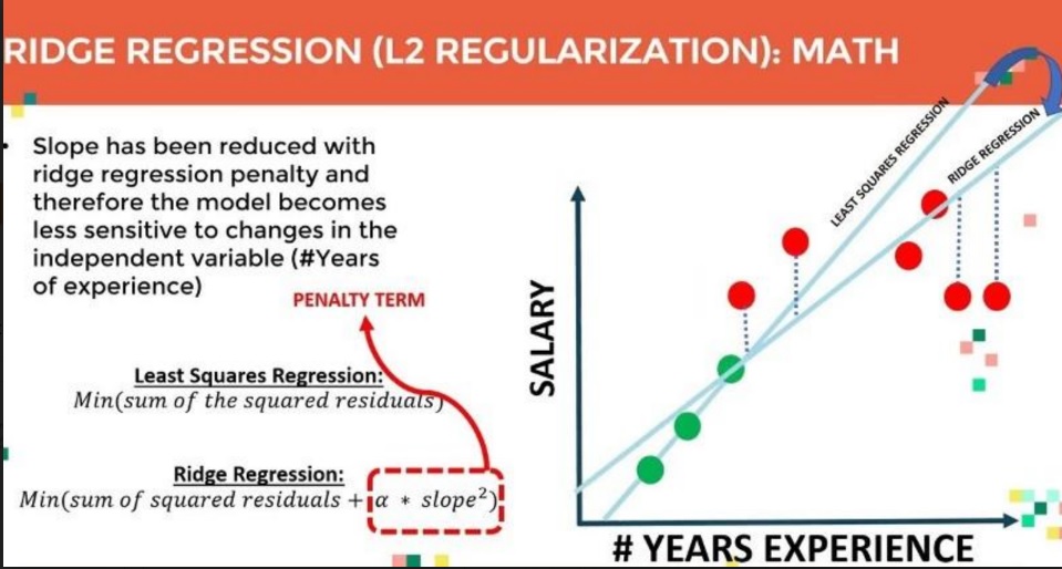
Ridge Regularization

Also known as Ridge Regression, it adjusts models with overfitting or underfitting by adding a penalty equivalent to the sum of the squares of the magnitudes of the coefficients.

This implies that we minimize the mathematical function representing our machine learning model and calculate the coefficients. We multiply and add the size of the coefficients. Ridge Regression performs regularization machine learning by reducing the coefficients present. The function shown below shows the cost function of the ridge regression.

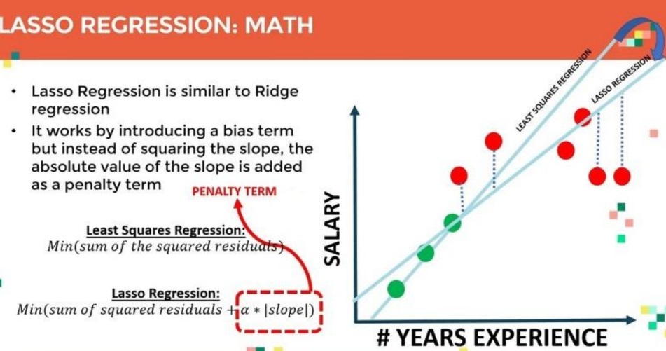
Lasso Regularization

Modifies overfitted or under-fitted models by adding a penalty equivalent to the sum of the absolute values ​​of the coefficients.

Lasso regression also performs coefficient minimization, but instead of squaring the magnitudes of the coefficients, it takes the actual values ​​of the coefficients. This means that the sum of the coefficients can also be 0 because there are negative coefficients. Consider the cost function for the lasso regression.

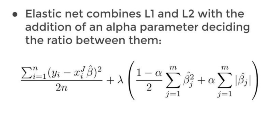
Elastic Net

Elastic Net combines L1 and L2 With the addition of an alpha Parameter.

Regularization Using Python in Machine Learning

Let’s see how regularisation can be implemented in Python. We have taken the Advertising Dataset on which we will use linear regression to predict Advertisement cost.

We start by importing all the necessary modules.

import numpy as np
import pandas as pd
import matplotlib.pyplot as plt
%matplotlib inline
import seaborn as sns

The Advertisement Dataset from sklearn’s datasets.

df = pd.read_csv("Advertising.csv")

Splitting the Dataset into Training and Testing Dataset:

Applying the Train Train Split:

Python Code:

import pandas as pd
from sklearn.model_selection import train_test_split

df = pd.read_csv("Advertising.csv")
X = df[["TV", "Radio", "Newspaper"]]
y = df["Sales"]
X_train, X_test, y_train, y_test = train_test_split(X, y, test_size = 0.3, random_state = 42)

print(X_train.shape, X_test.shape)

Now we can use them for training our linear regression model. We’ll start by creating our model and fitting the data into it. We then predict on the test set and find the error in our prediction using mean_squared_error. Finally, we print the coefficients of our linear regression model.

Ridge Regression:

 Modelling with default Parameters:

from sklearn.linear_model import Ridge
ridge_model = Ridge()
ridge_model.fit(X_train, y_train)

Predictions and Evaluation Of Ridge Regression:

test_predictions = ridge_model.predict(X_test)
train_predictions = ridge_model.predict(X_train)

Hyperparameter Tuning of Ridge :

Identifying the best alpha value for Ridge Regression:

from sklearn.model_selection import GridSearchCV
estimator = Ridge()
estimator = Ridge()
param_grid = {"alpha":list(range(1,11))}
model_hp = GridSearchCV(estimator, param_grid, cv = 5)
model_hp.fit(X_train, y_train)
model_hp.best_params_

Lasso Regularization:

Modeling of Lasso Regularization:

from sklearn.linear_model import Lasso
lasso_model = Lasso()
lasso_model.fit(X_train, y_train)

Predictions and Evaluation Of Lasso Regression:

test_predictions = lasso_model.predict(X_test)
train_predictions = lasso_model.predict(X_train)
from sklearn.metrics import mean_squared_error
train_rmse = np.sqrt(mean_squared_error(y_test, test_predictions))
test_rmse = np.sqrt(mean_squared_error(y_train, train_predictions))
print("train RMSE:", train_rmse)
print("test RMSE:", test_rmse)

Hyperparameter Tuning of Lasso: 

Identifying the best alpha value for Lasso Regression:

param_grid = {"alpha": list(range(1,11))}
model_hp = GridSearchCV(estimator, param_grid, cv =5)
model_hp.fit(X_train, y_train)
model_hp.best_estimator_

Elastic Net Regularization:

modeling of Elastic Net Regularization:

from sklearn.linear_model import ElasticNet
enr_model = ElasticNet(alpha=2, l1_ratio = 1)
enr_model.fit(X_train, y_train)

Predictions and Evaluation Of Elastic Net:

test_predictions = enr_model.predict(X_test)
train_predictions = enr_model.predict(X_train)
from sklearn.metrics import mean_squared_error
train_rmse = np.sqrt(mean_squared_error(y_test, test_predictions))
test_rmse = np.sqrt(mean_squared_error(y_train, train_predictions))
print("train RMSE:", train_rmse)
print("test RMSE:", test_rmse)

Hyperparameter Tuning of Elastic Net:

Identifying the best alpha value for Elastic Net:

from sklearn.model_selection import GridSearchCV
enr_hp = GridSearchCV(estimator, param_grid)
enr_hp.fit(X_train, y_train)
enr_hp.best_params_
param_grid = { "alpha" : [0, 0.1, 0.2, 1, 2, 3, 5, 10],
"l1_ratio" : [0.1, 0.5, 0.75, 0.9, 0.95, 1]}
estimator = ElasticNet()

Conclusion

In this article – The Ultimate Guide to Regularization in Machine Learning, we learned about the different ways models can become unstable by being under- or overfitted. We observed the role of bias and Variance. We then moved to regularization machine learning techniques to overcome overfitting and underfitting. and Finally, we Saw a Python Code Implementation.

Key Takeaways:

• We learned about the L1 and L2 Regularization, which are added to the cost function.
• In each of these algorithms, we can set to specify several hyperparameters.
• We can use GridSearchCV or the respective Hyperparameter Tuning algorithms of the given respective regression model to find the optimal hyperparameters.

The media shown in this article is not owned by Analytics Vidhya and is used at the Author’s discretion.

Frequently Asked Questions

ANURAG SINGH CHOUDHARY 07 Jun 2024