Coca-Cola Bottle Image Recognition (with Python code)
Introduction
THE DEPENDENCIES
import numpy as np
import pandas as pd
import matplotlib.pyplot as plt
from mpl_toolkits.mplot3d import Axes3D
from matplotlib import cm
from matplotlib import colors
import os
import cv2
import PIL
from tensorflow.keras.layers import Dense,Conv2D, Dropout,Flatten, MaxPooling2D
from tensorflow import keras
from tensorflow.keras.models import Sequential, save_model, load_model
from tensorflow.keras.optimizers import Adam
import tensorflow as tf
from tensorflow.keras.preprocessing.image import img_to_array
from tensorflow.keras.preprocessing.image import load_img
from tensorflow.keras.applications.inception_v3 import InceptionV3, preprocess_input
from tensorflow.keras.callbacks import ModelCheckpoint
from sklearn.decomposition import PCA
- Numpy is used to manipulate array data.
- Matplotlib is used to visualize the images and to show how discernable a color is in a particular range of colors.
- OS is used to access the file structure.
- CV2 is used to read the images and convert them into different color schemes.
- Keras is used for the actual Neural Network.
CONVERTING THE COLOR SCHEME
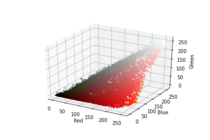
DETERMINING THE APPROPRIATE COLOR SCHEME:
red, green, blue = cv2.split(img)
fig = plt.figure()
axis = fig.add_subplot(1, 1, 1, projection="3d")
pixel_colors = img.reshape((np.shape(img)[0]*np.shape(img)[1], 3))
norm = colors.Normalize(vmin=-1.,vmax=1.)
norm.autoscale(pixel_colors)
pixel_colors = norm(pixel_colors).tolist()
axis.scatter(red.flatten(), green.flatten(), blue.flatten(), facecolors=pixel_colors, marker=".")
axis.set_xlabel("Red")
axis.set_ylabel("Green")
axis.set_zlabel("Blue")
plt.show()
hue, saturation, lightness = cv2.split(img)
fig = plt.figure()
axis = fig.add_subplot(1, 1, 1, projection="3d")
axis.scatter(hue.flatten(), saturation.flatten(), lightness.flatten(), facecolors=pixel_colors, marker=".")
axis.set_xlabel("Hue")
axis.set_ylabel("Saturation")
axis.set_zlabel("Lightness")
plt.show()
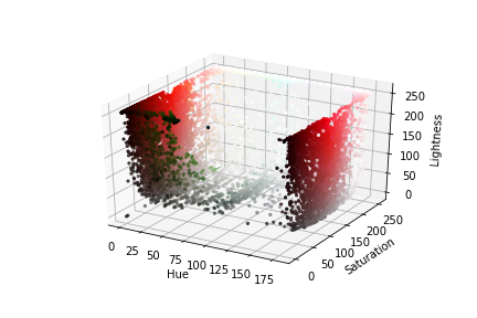
To note is that particular colors are not as jumbled up in the second plot as in the first. We can easily discern the white color pixels from the rest.
CONVERTING THE COLORS
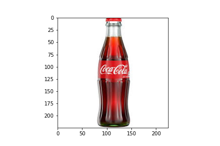
img = cv2.imread(img_path)
plt.imshow(img)
plt.show()
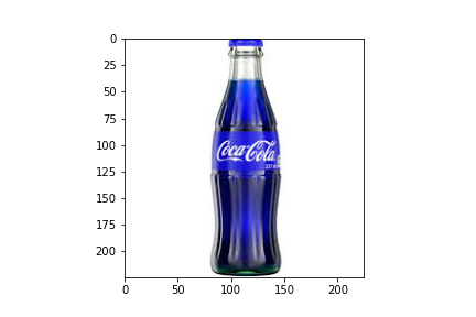
img = cv2.cvtColor(img, cv2.COLOR_BGR2RGB)
plt.imshow(img)
plt.show()
img = cv2.cvtColor(img, cv2.COLOR_RGB2HLS)
plt.imshow(img)
plt.show()
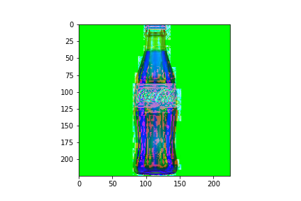
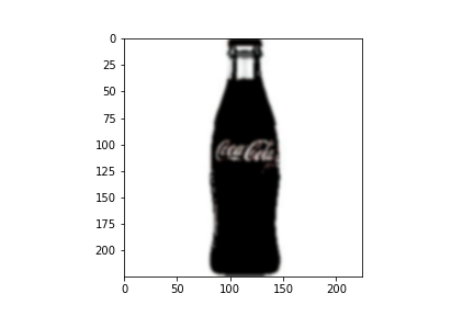
ISOLATE COLOR WHITE:
 hsl_img = cv2.cvtColor(img, cv2.COLOR_RGB2HLS)
 low_threshold = np.array([0, 200, 0], dtype=np.uint8)
 high_threshold = np.array([180, 255, 255], dtype=np.uint8)
 mask = cv2.inRange(hsl_img, low_threshold, high_threshold)
 white_parts = cv2.bitwise_and(img, img, mask = mask)
 blur = cv2.GaussianBlur(white_parts, (7,7), 0)
TRANSFER LEARNING WITH INCEPTIONV3
model = InceptionV3(weights='imagenet', include_top=False, input_shape=(299, 299, 3))
bottle_neck_features_train = model.predict_generator(X, n/32, verbose=1)
bottle_neck_features_train.shape
np.savez('inception_features_train', features=bottle_neck_features_train)
train_data = np.load('inception_features_train.npz')['features']
train_labels = np.array([0] * m + [1] * p) // where m+p = n
THE NEURAL NETWORK
classifier = Sequential()
classifier.add(Conv2D(32, (3, 3), activation='relu', input_shape=train_data.shape[1:], padding='same'))
classifier.add(Conv2D(32, (3, 3), activation='relu', padding='same'))
classifier.add(MaxPooling2D(pool_size=(3, 3)))
classifier.add(Dropout(0.25))
classifier.add(Conv2D(64, (3, 3), activation='relu', padding='same'))
classifier.add(Conv2D(64, (3, 3), activation='relu', padding='same'))
classifier.add(MaxPooling2D(pool_size=(2, 2)))
classifier.add(Dropout(0.50))
classifier.add(Flatten())
classifier.add(Dense(512, activation='relu'))
classifier.add(Dropout(0.6))
classifier.add(Dense(256, activation='relu'))
classifier.add(Dropout(0.5))
classifier.add(Dense(1, activation='sigmoid'))
checkpointer = ModelCheckpoint(filepath='./weights_inception.hdf5', verbose=1, save_best_only=True)
classifier.compile(optimizer='adam',loss='binary_crossentropy',metrics=['binary_accuracy'])
history = classifier.fit(train_data, train_labels,epochs=50,batch_size=32, validation_split=0.3,  verbose=2, callbacks=[checkpointer], shuffle=True)
PERFORMING PREDICTIONS
def predict(filepath):
    img = cv2.imread(filepath)
    img = cv2.resize(img,(299,299))
    img = cv2.cvtColor(img, cv2.COLOR_BGR2RGB)
    hsl_img = cv2.cvtColor(img, cv2.COLOR_RGB2HLS)
    low_threshold = np.array([0, 200, 0], dtype=np.uint8)
    high_threshold = np.array([180, 255, 255], dtype=np.uint8)
    mask = cv2.inRange(hsl_img, low_threshold, high_threshold)
    white_parts = cv2.bitwise_and(img, img, mask = mask)
    blur = cv2.GaussianBlur(white_parts, (7,7), 0)
    print(img.shape)
    clf = InceptionV3(weights='imagenet', include_top=False, input_shape=white_parts.shape)
    bottle_neck_features_predict = clf.predict(np.array([white_parts]))[0]
    np.savez('inception_features_prediction', features=bottle_neck_features_predict)
    prediction_data = np.load('inception_features_prediction.npz')['features']
    q = model.predict( np.array( [prediction_data,] )  )
    prediction = q[0]
    prediction = int(prediction)
    print(prediction)
NEXT STEPS
Seeing as how we have the following:
- A working predictive model.
- Saved values for the model.
- Images for prediction.
- A function ready for making predictions.
We can now try and perform predictions on images.
All we need to do is to call the predict function and pass the path to the image as a parameter.
predict("./train/Coke Bottles/Coke1.png")
This should provide 1 as an output since our images of coke bottles we labeled as 1.
SAVING THE MODEL
If this is to be at all applicable in software such as a real-time app that uses OpenCV modules to view an image or video and make predictions, we cannot realistically hope to train our model every time the program is turned on.
Much more logical is to save the model and load it up once the program is opened. This means we need to make use of Keras’ load_model and save_model. We import these as follows.
from tensorflow.keras.models import Sequential, save_model, load_model
Now we can save the model by calling save_model() and entering the folder name as a parameter.
save_model(save_model)
Finally, we can tidy up any program by simply loading the model using load_model rather than entering the code to re-train the model.
load_model("./save_model")
The media shown in this article are not owned by Analytics Vidhya and is used at the Author’s discretion.


