Topic Modeling: Predicting Multiple Tags of Research Articles using OneVsRest strategy

Recently I participated in an NLP hackathon — “Topic Modeling for Research Articles 2.0”. This hackathon was hosted by the Analytics Vidhya platform as a part of their HackLive initiative. The participants were guided by experts in a 2-hour live session and later on were given a week to compete and climb the leaderboard.
Problem Statement
Given the abstracts for a set of research articles, the task is to predict the tags for each article included in the test set.
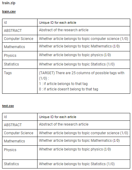
The research article abstracts are sourced from the following 4 topics — Computer Science, Mathematics, Physics, Statistics. Each article can possibly have multiple tags among 25 tags like Number Theory, Applications, Artificial Intelligence, Astrophysics of Galaxies, Information Theory, Materials Science, Machine Learning et al. Submissions are evaluated on micro F1 Score between the predicted and observed tags for each article in the test set.
Complete Problem Statement and the dataset is available here.
Without further ado let’s get started with the code.
Loading and Exploring data
Importing necessary libraries —
%matplotlib inline
import numpy as np
import pandas as pd
import matplotlib.pyplot as plt
import seaborn as sns
#-----------------------------------
from nltk.tokenize import word_tokenize
from nltk.stem import PorterStemmer
#-----------------------------------
from sklearn.feature_extraction.text import CountVectorizer
from sklearn.feature_extraction.text import TfidfVectorizer
#-----------------------------------
from sklearn import metrics
from sklearn.metrics import accuracy_score
from sklearn.metrics import f1_score
Load train and test data from .csv files into Pandas DataFrame —
train_data = pd.read_csv(‘Train.csv’)
test_data = pd.read_csv(‘Test.csv’)
Train and Test data shape —
print(“Train size:”, train_data.shape)
print(“Test size:”, test_data.shape)
Output:
![]()
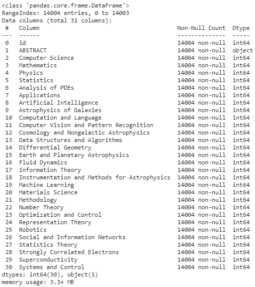
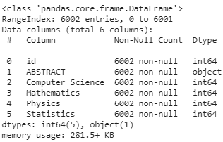
There are ~ 14k datapoints in the Train dataset and ~6k datapoints in the Test set. Overview of train and test datasets —
train_data.info()
Output:
test_data.info()
Output:
As we can see from the train data info, there are 31 columns — 1 column for id, 1 column for Abstract text, 4 columns for topics, these all form our feature variables, and the next 25 columns are class-labels that we have to ‘learn’ for the prediction task.
topic_cols = [‘Computer Science’, ‘Mathematics’, ‘Physics’, ‘Statistics’]
target_cols = [‘Analysis of PDEs’, ‘Applications’, ‘Artificial Intelligence’, ‘Astrophysics of Galaxies’, ‘Computation and Language’, ‘Computer Vision and Pattern Recognition’, ‘Cosmology and Nongalactic Astrophysics’, ‘Data Structures and Algorithms’, ‘Differential Geometry’, ‘Earth and Planetary Astrophysics’, ‘Fluid Dynamics’, ‘Information Theory’, ‘Instrumentation and Methods for Astrophysics’, ‘Machine Learning’, ‘Materials Science’, ‘Methodology’, ‘Number Theory’, ‘Optimization and Control’, ‘Representation Theory’, ‘Robotics’, ‘Social and Information Networks’, ‘Statistics Theory’, ‘Strongly Correlated Electrons’, ‘Superconductivity’, ‘Systems and Control’]
How many datapoints have more than 1 tags?
my_list = []
for i in range(train_data.shape[0]):
    my_list.append(sum(train_data.iloc[i, 6:]))
pd.Series(my_list).value_counts()
Output:
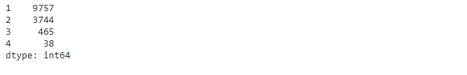
So, most of our research articles have either 1 or 2 tags.
Data cleaning and preprocessing for OneVsRest Classifier
Before proceeding with data cleaning and pre-processing, it’s a good idea to first print and observe some random samples from training data in order to get an overview. Based on my observation I built the below pipeline for cleaning and pre-processing the text data:
De-contraction → Removing special chars → Removing stopwords →Stemming
First, we define some helper functions needed for text processing.
De-contracting the English phrases —
def decontracted(phrase):
  #specific
  phrase = re.sub(r”won’t”, “will not”, phrase)
  phrase = re.sub(r”can’t”, “cannot”, phrase)
  # general
  phrase = re.sub(r”n’t”, “ not”, phrase)
  phrase = re.sub(r”’re”, “ are”, phrase)
  phrase = re.sub(r”’s”, “ is”, phrase)
  phrase = re.sub(r”’d”, “ would”, phrase)
  phrase = re.sub(r”’ll”, “ will”, phrase)
  phrase = re.sub(r”’t”, “ not”, phrase)
  phrase = re.sub(r”’ve”, “ have”, phrase)
  phrase = re.sub(r”’m”, “ am”, phrase)
  phrase = re.sub(r”’em”, “ them”, phrase)
  return phrase
Declare stopwords —
(I prefer my own custom set of stopwords to the in-built ones. It helps to me readily modify the stopwords set depending on the problem)
stopwords = [‘i’, ‘me’, ‘my’, ‘myself’, ‘we’, ‘our’, ‘ours’, ‘ourselves’, ‘you’, “you’re”, “you’ve”, “you’ll”, “you’d”, ‘your’, ‘yours’, ‘yourself’, ‘yourselves’, ‘he’, ‘him’, ‘his’, ‘himself’, ‘she’, “she’s”, ‘her’, ‘hers’, ‘herself’, ‘it’, “it’s”, ‘its’, ‘itself’, ‘they’, ‘them’, ‘their’, ‘theirs’, ‘themselves’, ‘what’, ‘which’, ‘who’, ‘whom’, ‘this’, ‘that’, “that’ll”, ‘these’, ‘those’, ‘am’, ‘is’, ‘are’, ‘was’, ‘were’, ‘be’, ‘been’, ‘being’, ‘have’, ‘has’, ‘had’, ‘having’, ‘do’, ‘does’, ‘did’, ‘doing’, ‘a’, ‘an’, ‘the’, ‘and’, ‘but’, ‘if’, ‘or’, ‘because’, ‘as’, ‘until’, ‘while’, ‘of’, ‘at’, ‘by’, ‘for’, ‘with’, ‘about’, ‘against’, ‘between’, ‘into’, ‘through’, ‘during’, ‘before’, ‘after’, ‘above’, ‘below’, ‘to’, ‘from’, ‘up’, ‘down’, ‘in’, ‘out’, ‘on’, ‘off’, ‘over’, ‘under’, ‘again’, ‘further’, ‘then’, ‘once’, ‘here’, ‘there’, ‘when’, ‘where’, ‘why’, ‘how’, ‘all’, ‘any’, ‘both’, ‘each’, ‘few’, ‘more’, ‘most’, ‘other’, ‘some’, ‘such’, ‘only’, ‘own’, ‘same’, ‘so’, ‘than’, ‘too’, ‘very’, ‘s’, ‘t’, ‘can’, ‘will’, ‘just’, ‘don’, “don’t”, ‘should’, “should’ve”, ‘now’, ‘d’, ‘ll’, ‘m’, ‘o’, ‘re’, ‘ve’, ‘y’, ‘ain’, ‘aren’, “aren’t”, ‘couldn’, “couldn’t”, ‘didn’, “didn’t”, ‘doesn’, “doesn’t”, ‘hadn’, “hadn’t”, ‘hasn’, “hasn’t”, ‘haven’, “haven’t”, ‘isn’, “isn’t”, ‘ma’, ‘mightn’, “mightn’t”, ‘mustn’, “mustn’t”, ‘needn’, “needn’t”, ‘shan’, “shan’t”, ‘shouldn’, “shouldn’t”, ‘wasn’, “wasn’t”, ‘weren’, “weren’t”, ‘won’, “won’t”, ‘wouldn’, “wouldn’t”]
Alternatively, you can directly import stopwords from word cloud API —
from wordcloud import WordCloud, STOPWORDS
stopwords = set(list(STOPWORDS))
Stemming using Porter stemmer —
def stemming(sentence):
  token_words = word_tokenize(sentence)
  stem_sentence = []
  for word in token_words:
    stemmer = PorterStemmer()
    stem_sentence.append(stemmer.stem(word))
    stem_sentence.append(“ “)
  return “”.join(stem_sentence)
Now that we’ve defined all the functions, let’s write a text pre-processing pipeline —
def text_preprocessing(text):
  preprocessed_abstract = []
  for sentence in text:
    sent = decontracted(sentence)
    sent = re.sub(‘[^A-Za-z0–9]+’, ‘ ‘, sent)
    sent = ‘ ‘.join(e.lower() for e in sent.split() if e.lower() not in stopwords)
    sent = stemming(sent)
    preprocessed_abstract.append(sent.strip())
  return preprocessed_abstract
Preprocessing the train data abstract text—
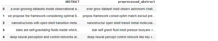
train_data[‘preprocessed_abstract’] = text_preprocessing(train_data[‘ABSTRACT’].values)
train_data[[‘ABSTRACT’, ‘preprocessed_abstract’]].head()
Output:
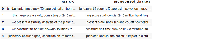
Likewise, preprocessing the test dataset –
test_data[‘preprocessed_abstract’] = text_preprocessing(test_data[‘ABSTRACT’].values)
test_data[[‘ABSTRACT’, ‘preprocessed_abstract’]].head()
Output:
Now we longer need the original ‘ABSTRACT’ column. You may drop this column from the datasets.
Text data encoding
Splitting train data into train and validation datasets —
X = train_data[[‘Computer Science’, ‘Mathematics’, ‘Physics’, ‘Statistics’, ‘preprocessed_abstract’]]
y = train_data[target_cols]

from sklearn.model_selection import train_test_split
X_train, X_cv, y_train, y_cv = train_test_split(X, y, test_size = 0.25, random_state = 21)
print(X_train.shape, y_train.shape)
print(X_cv.shape, y_cv.shape)
Output:
![]()
As we can see, we have got ~ 10500 datapoints in our training set and ~3500 datapoints in the validation set.
TF-IDF vectorization of text data
Building vocabulary —
combined_vocab = list(train_data[‘preprocessed_abstract’])
                 + list(test_data[‘preprocessed_abstract’])
Yes, here I’ve knowingly committed a sin! I have used the complete train and test data for building vocabulary to train a model on it. Ideally, your model shouldn’t be seeing the test data.
vectorizer = TfidfVectorizer(min_df = 5, max_df = 0.5, sublinear_tf = True, ngram_range = (1, 1))
vectorizer.fit(combined_vocab)
X_train_tfidf = vectorizer.transform(X_train[‘preprocessed_abstract’])

X_cv_tfidf = vectorizer.transform(X_cv[‘preprocessed_abstract’])
print(X_train_tfidf.shape, y_train.shape)
print(X_cv_tfidf.shape, y_cv.shape)
Output:
![]()
After TF-IDF encoding we obtain 9136 features, each of them corresponding to a distinct word in the vocabulary.
Some important things you should know here —
- I didn’t directly jump to a conclusion that I should go with TF-IDF vectorization. I tried different methods like BOW, W2V using a pre-trained GloVe model, etc. Among them, TF-IDF turned out to be the best performing so here I’m demonstrating only this.
- It didn’t magically appear to me that I should be going with uni-grams. I tried bi-grams, tri-grams, and even four-grams; the model employing the unigrams gave the best performance among all.
Text data encoding is a tricky thing. Especially in competitions where even a difference of 0.001 in the performance metric can push you several places behind on the leaderboard. So, one should be open to trying different permutations & combinations at a rudimentary stage.
Before we proceed with modeling, we stack all the features(topic features + TF-IDF encoded text features) together for both train and test datasets respectively.
from scipy.sparse import hstack
X_train_data_tfidf = hstack((X_train[topic_cols], X_train_tfidf))
X_cv_data_tfidf = hstack((X_cv[topic_cols], X_cv_tfidf))
Multi-label classification using OneVsRest Classifier
Until now we were only dealing with refining and vectorizing the feature variables. As we know, this is a multi-label classification problem and each document may have one or more predefined tags simultaneously. We already saw that several datapoints have 2 or 3 tags.
Most traditional machine learning algorithms are developed for single-label classification problems. Therefore a lot of approaches in the literature transform the multi-label problem into multiple single-label problems so that the existing single-label algorithms can be used.
One such technique is One-vs-the-rest (OvR) multiclass/multilabel classifier, also known as one-vs-all. In OneVsRest Classifier, we fit one classifier per class and it is the most commonly used strategy for multiclass/multi-label classification and is a fair default choice. For each classifier, the class is fitted against all the other classes. In addition to its computational efficiency, one advantage of this approach is its interpretability. Since each class is represented by one and one classifier only, it is possible to gain knowledge about the class by inspecting its corresponding classifier.
Let’s search for the optimal hyper-parameter ‘C’ —
(‘C’ denotes inverse of regularization strength. Smaller values specify stronger regularization).
from sklearn.multiclass import OneVsRestClassifier
from sklearn.linear_model import LogisticRegression
C_range = [0.01, 0.1, 1, 10, 100] for i in C_range:
  clf = OneVsRestClassifier(LogisticRegression(C = i, solver =  ‘sag’))
  clf.fit(X_train_data_tfidf, y_train)
  y_pred_train = clf.predict(X_train_data_tfidf)
  y_pred_cv = clf.predict(X_cv_data_tfidf)
  f1_score_train = f1_score(y_train, y_pred_train, average = ‘micro’)
  f1_score_cv = f1_score(y_cv, y_pred_cv, average = ‘micro’)
  print(“C:”, i, “Train Score:”,f1_score_train, “CV Score:”, f1_score_cv)
 print(“- “*50)
Output:
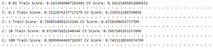
We can see that the highest validation score is obtained at C = 10. But the training score here is also very high, which was kind of expected.
Let’s tune the hyper-parameter even further —
from sklearn.multiclass import OneVsRestClassifier
from sklearn.linear_model import LogisticRegressionC_range = [10, 20, 40, 70, 100]
for i in C_range:
  clf = OneVsRestClassifier(LogisticRegression(C = i, solver =  ‘sag’))
  clf.fit(X_train_data_tfidf, y_train)
  y_pred_train = clf.predict(X_train_data_tfidf)
  y_pred_cv = clf.predict(X_cv_data_tfidf)
  f1_score_train = f1_score(y_train, y_pred_train, average = ‘micro’)
  f1_score_cv = f1_score(y_cv, y_pred_cv, average = ‘micro’)
  print(“C:”, i, “Train Score:”,f1_score_train, “CV Score:”, f1_score_cv)
 print(“- “*50)
Output:
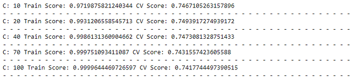
The model with C = 20 gives the best score on the validation set. So, going further, we take C = 20.
If you notice, here we have used the default L2 penalty for regularization as the model with L2 gave me the best result among L1, L2, and elastic-net mixing.
Determining the right thresholds for OneVsRest Classifier
The default threshold in binary classification algorithms is 0.5. But this may not be the best threshold given the data and the performance metrics that we intend to maximize. As we know, the F1 score is given by —
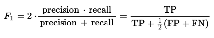
A good threshold(for each distinct label) would be the one that maximizes the F1 score.
def get_best_thresholds(true, pred):
  thresholds = [i/100 for i in range(100)]
  best_thresholds = []
  for idx in range(25):
    f1_scores = [f1_score(true[:, idx], (pred[:, idx] > thresh) * 1) for thresh in thresholds]
    best_thresh = thresholds[np.argmax(f1_scores)]
    best_thresholds.append(best_thresh)
 return best_thresholds
In a nutshell, what the above function does is, for each of the 25 class labels, it computes the F1 scores corresponding to each of the hundred thresholds and then selects that threshold which returns the maximum F1 score for the given class label.
If the individual F1 score is high, the micro-average F1 will also be high. Let’s get the thresholds —
clf = OneVsRestClassifier(LogisticRegression(C = 20, solver = ‘sag’))
clf.fit(X_train_data_tfidf, y_train)
y_pred_train_proba = clf.predict_proba(X_train_data_tfidf)
y_pred_cv_proba = clf.predict_proba(X_cv_data_tfidf)
best_thresholds = get_best_thresholds(y_cv.values, y_pred_cv_proba)
print(best_thresholds)
Output:
[0.45, 0.28, 0.19, 0.46, 0.24, 0.24, 0.24, 0.28, 0.22, 0.2, 0.22, 0.24, 0.24, 0.41, 0.32, 0.15, 0.21, 0.33, 0.33, 0.29, 0.16, 0.66, 0.33, 0.36, 0.4]
As you can see we have obtained a distinct threshold value for each class label. We’re going to use these same values in our final OneVsRest Classifier model. Making predictions using the above thresholds —
y_pred_cv = np.empty_like(y_pred_cv_proba)for i, thresh in enumerate(best_thresholds):
  y_pred_cv[:, i] = (y_pred_cv_proba[:, i] > thresh) * 1
  print(f1_score(y_cv, y_pred_cv, average = ‘micro’))
Output:
0.7765116517811312
Thus, we have managed to obtain a significantly better score using the variable thresholds.
So far we have performed hyper-parameter tuning on the validation set and managed to obtain the optimal hyperparameter (C = 20). Also, we tweaked the thresholds and obtained the right set of thresholds for which the F1 score is maximum.
Making a prediction on the test data using OneVsRest Classifier
Using the above parameters let’s move on to build train a full-fledged model on the entire training data and make a prediction on the test data.
# train and test data
X_tr = train_data[[‘Computer Science’, ‘Mathematics’, ‘Physics’, ‘Statistics’, ‘preprocessed_abstract’]]
y_tr = train_data[target_cols]
X_te = test_data[[‘Computer Science’, ‘Mathematics’, ‘Physics’, ‘Statistics’, ‘preprocessed_abstract’]]

# text data encoding
vectorizer.fit(combined_vocab)
X_tr_tfidf = vectorizer.transform(X_tr['preprocessed_abstract'])
X_te_tfidf = vectorizer.transform(X_te['preprocessed_abstract'])

# stacking
X_tr_data_tfidf = hstack((X_tr[topic_cols], X_tr_tfidf))
X_te_data_tfidf = hstack((X_te[topic_cols], X_te_tfidf))

# modeling and making prediction with best thresholds
clf = OneVsRestClassifier(LogisticRegression(C = 20))
clf.fit(X_tr_data_tfidf, y_tr)
y_pred_tr_proba = clf.predict_proba(X_tr_data_tfidf)
y_pred_te_proba = clf.predict_proba(X_te_data_tfidf)
y_pred_te = np.empty_like(y_pred_te_proba)
for i, thresh in enumerate(best_thresholds):
  y_pred_te[:, i] = (y_pred_te_proba[:, i] > thresh) * 1
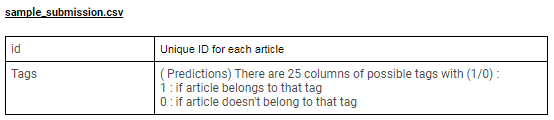
Once we obtain our test predictions, we attach them to the respective ids (as in the sample submission file) and make a submission in the designated format.
ss = pd.read_csv(‘SampleSubmission.csv’)
ss[target_cols] = y_pred_te
ss.to_csv(‘LR_tfidf10k_L2_C20.csv’, index = False)
The best thing about participating in the hackathons is that you get to experiment with different techniques, so when you encounter similar kind of problem in the future you have a fair understanding of what works and what doesn’t. And also you get to learn a lot from other participants by actively participating in the discussions.
You can find the complete code here on my GitHub profile.
About the Author
Pratik Nabriya is a skilled Data Professional currently employed with an Analytics & AI firm based out of Noida. He is proficient in Machine learning, Deep learning, NLP, Time-Series Analysis, SQL, Data manipulation & Visualisation and is familiar with working in a Cloud environment. In his spare time, he loves to compete in Hackathons, and write blogs & articles at the crossroads of Data & Finance.


