Stock Market Forecasting using Time Series Analysis with ARIMA Model

Introduction

The stock market is a marketplace that allows for the seamless exchange of corporate stock purchases and sales. Every Stock Exchange has its own value for the Stock Index. The index is the average value derived by adding up the prices of various equities. This aids in the representation of the entire stock market as well as the forecasting of market movement over time. The stock market can have a significant impact on individuals and the economy as a whole. As a result, effectively predicting stock market trends can reduce the risk of loss while increasing profit through stock market prediction.

We will use the ARIMA model to forecast the stock price of ARCH CAPITAL GROUP in this tutorial, focusing on various trading strategies and machine learning algorithms to handle market data effectively. The application of these techniques aims to manage the low predictability and volatility within financial markets.

Learning Objectives

• Learn how the Autoregressive Integrated Moving Average (ARIMA) model utilizes historical data to forecast future stock market prices and stock returns.
• Gain practical experience in applying ARIMA methodology to real-world stock data to identify trends and seasonal patterns in stock market movements.
• Develop skills to assess the accuracy of ARIMA model predictions using common statistical metrics like MSE, MAE, RMSE, and MAPE, enhancing your ability to make informed trading strategies.

This article was published as a part of the Data Science Blogathon.

What is ARIMA Model?

The Autoregressive Integrated Moving Average (ARIMA) model is a powerful predictive tool used primarily in time series analysis. This model is crucial for transforming non-stationary data into stationary data, a necessary step for effective forecasting. ARIMA is renowned for its application in predicting future prices based on historical data, making it highly valued in financial sectors such as banking and economics. By using regression on past values, ARIMA helps to accurately forecast short-term movements in stock prices and stock returns, demonstrating its efficacy as a predictive model.

ARIMA’s Role in Forecasting Market Prices

ARIMA excels in the stock market by analyzing historical data to predict future stock prices, thereby aiding in short-term investment decisions. It integrates three essential components: Autoregression (AR), Differencing (I), and Moving Average (MA). The AR component models the relationship between a stock’s current price and its historical prices. Differencing helps stabilize the series by mitigating variations at different lags, essential for maintaining stationarity. The MA aspect manages the noise in the data by smoothing out past forecast errors. Collectively, these features enable ARIMA to provide robust predictions of market prices, capturing the dynamic patterns and trends inherent in time series data of stock returns.

We will use the ARIMA model to forecast the stock price of ARCH CAPITAL GROUP in this tutorial.

Load Required Libraries

!pip install pmdarima
import os
import warnings
warnings.filterwarnings('ignore')
import numpy as np
import pandas as pd
import matplotlib.pyplot as plt
from statsmodels.tsa.stattools import adfuller
from statsmodels.tsa.seasonal import seasonal_decompose
from statsmodels.tsa.arima.model import ARIMA
from pmdarima.arima import auto_arima
from sklearn.metrics import mean_squared_error, mean_absolute_error
import math

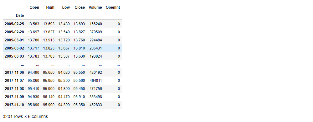
stock_data = pd.read_csv(
    'acgl.us.txt', 
    sep=',', 
    index_col='Date', 
    parse_dates=['Date'], 
    date_parser=lambda dates: pd.to_datetime(dates, format='%Y-%m-%d')  ).fillna(0)
stock_data

Output:

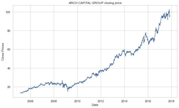
Visualize the Stock’s Daily Closing Price

#plot close price
plt.figure(figsize=(10,6))
plt.grid(True)
plt.xlabel('Date')
plt.ylabel('Close Prices')
plt.plot(stock_data['Close'])
plt.title('ARCH CAPITAL GROUP closing price')
plt.show()

Output:

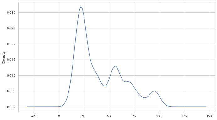
We can also use a probability distribution to visualize the data in our series.

#Distribution of the dataset
df_close = stock_data['Close']
df_close.plot(kind='kde')

Output:

Test for Stationarity

A time series is also regarded to include three systematic components: level, trend, and seasonality, as well as one non-systematic component termed noise. The following are the components’ definitions:

• The average value in the series is called the level.
• The increasing or falling value in the series is referred to as the trend.
• Seasonality is the series’ recurring short-term cycle.
• The random variance in the series is referred to as noise.

Because time series analysis only works with stationary data, we must first determine whether a series is stationary.

Before proceeding, it is essential to understand the concept of stationarity in time series. A stationarity in a time series means that its statistical properties like mean and variance do not change over time. This stability is crucial because most forecasting models require the series to be stationary to produce reliable results. Non-stationary series, which show trends or seasonal variations, often need adjustments such as differencing or transformation to achieve stationarity.

ADF (Augmented Dickey-Fuller) Test

One of the most widely used statistical tests is the Dickey-Fuller test. It can be used to determine whether or not a series has a unit root, and thus whether or not the series is stationary. This test’s null and alternate hypotheses are:

• Null Hypothesis: The series has a unit root (value of a =1)
• Alternate Hypothesis: The series has no unit root.

If the null hypothesis is not rejected, the series is said to be non-stationary. The series can be linear or difference stationary as a result of this.

The series becomes stationary if both the mean and standard deviation are flat lines (constant mean and constant variance).

#Test for staionarity
def test_stationarity(timeseries):
    #Determing rolling statistics
    rolmean = timeseries.rolling(12).mean()
    rolstd = timeseries.rolling(12).std()
    #Plot rolling statistics:
    plt.plot(timeseries, color='blue',label='Original')
    plt.plot(rolmean, color='red', label='Rolling Mean')
    plt.plot(rolstd, color='black', label = 'Rolling Std')
    plt.legend(loc='best')
    plt.title('Rolling Mean and Standard Deviation')
    plt.show(block=False)
    print("Results of dickey fuller test")
    adft = adfuller(timeseries,autolag='AIC')
    # output for dft will give us without defining what the values are.
    #hence we manually write what values does it explains using a for loop
    output = pd.Series(adft[0:4],index=['Test Statistics','p-value','No. of lags used','Number of observations used'])
    for key,values in adft[4].items():
        output['critical value (%s)'%key] =  values
    print(output)
test_stationarity(df_close)

Output:

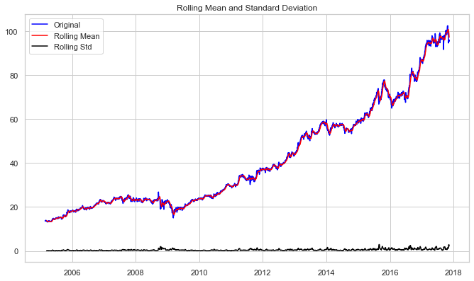
Results of dickey fuller test
Test Statistics                   1.374899
p-value                           0.996997
No. of lags used                  5.000000
Number of observations used    3195.000000
critical value (1%)              -3.432398
critical value (5%)              -2.862445
critical value (10%)             -2.567252
dtype: float64

We can also use a probability distribution to visualize the data in our series.

#Distribution of the dataset
df_close = stock_data['Close']
df_close.plot(kind='kde')

Output:

The increasing mean and standard deviation may be seen in the graph above, indicating that our series isn’t stationary.

We can’t rule out the Null hypothesis because the p-value is bigger than 0.05. Additionally, the test statistics exceed the critical values. As a result, the data is nonlinear.

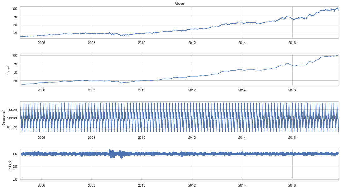
Eliminate Trend and Seasonality

Seasonality and trend may need to be separated from our series before we can undertake a time series analysis. This approach will cause the resulting series to become stagnant.

Let’s isolate the time series from the Trend and Seasonality.

#To separate the trend and the seasonality from a time series, 
# we can decompose the series using the following code.
result = seasonal_decompose(df_close, model='multiplicative', freq = 30)
fig = plt.figure()  
fig = result.plot()  
fig.set_size_inches(16, 9)

Output:

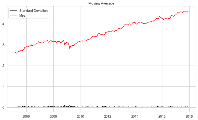
To reduce the magnitude of the values and the growing trend in the series, we first take a log of the series. We then calculate the rolling average of the series after obtaining the log of the series. A rolling average is computed by taking data from the previous 12 months and calculating a mean consumption value at each subsequent point in the series.

#if not stationary then eliminate trend
#Eliminate trend
from pylab import rcParams
rcParams['figure.figsize'] = 10, 6
df_log = np.log(df_close)
moving_avg = df_log.rolling(12).mean()
std_dev = df_log.rolling(12).std()
plt.legend(loc='best')
plt.title('Moving Average')
plt.plot(std_dev, color ="black", label = "Standard Deviation")
plt.plot(moving_avg, color="red", label = "Mean")
plt.legend()
plt.show()

Output:

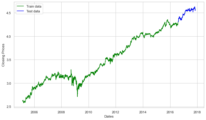
Split Data into Training and Test Sets

Now we’ll develop an ARIMA model and train it using the stock’s closing price from the train data. So, let’s visualize the data by dividing it into training and test sets.

#split data into train and training set
train_data, test_data = df_log[3:int(len(df_log)*0.9)], df_log[int(len(df_log)*0.9):]
plt.figure(figsize=(10,6))
plt.grid(True)
plt.xlabel('Dates')
plt.ylabel('Closing Prices')
plt.plot(df_log, 'green', label='Train data')
plt.plot(test_data, 'blue', label='Test data')
plt.legend()

Output:

It’s time to choose the ARIMA model’s p,q, and d parameters. We chose the values of p,d, and q last time by looking at the ACF and PACF charts, but this time we’ll utilize Auto ARIMA to find the best parameters without looking at the ACF and PACF graphs.

To clarify, the p parameter in the ARIMA model denotes the number of lag observations included in the model, reflecting the autoregressive part that predicts future values based on past values. The d parameter represents the degree of differencing required to make the data stationary, addressing trends or seasonal effects by subtracting previous observations from current ones. Lastly, q indicates the size of the moving average window, which incorporates the dependency of an observation on a residual error from a moving average model applied to lagged observations. Understanding these parameters is crucial as they directly impact the model’s ability to capture the underlying patterns in the time series data.

Auto ARIMA: Find the Best Parameters

The auto_arima function returns a fitted ARIMA model after determining the most optimal parameters for an ARIMA model. This function is based on the forecast::auto. Arima R function, which is widely used.

The auro_arima function works by performing differencing tests (e.g., Kwiatkowski–Phillips–Schmidt–Shin, Augmented Dickey-Fuller, or Phillips–Perron) to determine the order of differencing, d, and then fitting models within start p, max p, start q, max q ranges. After conducting the Canova-Hansen to determine the optimal order of seasonal differencing, D, auto_arima also seeks to identify the optimal P and Q hyper-parameters if the seasonal option is enabled.

model_autoARIMA = auto_arima(train_data, start_p=0, start_q=0,
                      test='adf',       # use adftest to find optimal 'd'
                      max_p=3, max_q=3, # maximum p and q
                      m=1,              # frequency of series
                      d=None,           # let model determine 'd'
                      seasonal=False,   # No Seasonality
                      start_P=0, 
                      D=0, 
                      trace=True,
                      error_action='ignore',  
                      suppress_warnings=True, 
                      stepwise=True)
print(model_autoARIMA.summary())
model_autoARIMA.plot_diagnostics(figsize=(15,8))
plt.show()

Output:

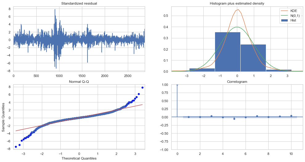
So, how should the plot diagnostics be interpreted?

Top left: The residual errors appear to have a uniform variance and fluctuate around a mean of zero.

Top Right: The density plot on the top right suggests a normal distribution with a mean of zero.

Bottom left: The red line should be perfectly aligned with all of the dots. Any significant deviations would indicate a skewed distribution.

Bottom Right: The residual errors are not autocorrelated, as shown by the Correlogram, also known as the ACF plot. Any autocorrelation would imply that the residual errors have a pattern that isn’t explained by the model. As a result, you’ll need to add more Xs (predictors) to the model.

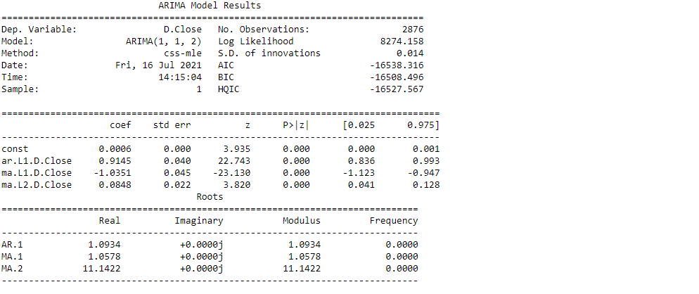
As a result, the Auto ARIMA model assigned the values 1, 1, and 2 to, p, d, and q, respectively.

As a result, the Auto ARIMA model assigned the values 1, 1, and 2 to, p, d, and q, respectively.

#Modeling
# Build Model
model = ARIMA(train_data, order=(1,1,2))  
fitted = model.fit(disp=-1)  
print(fitted.summary())

Output:

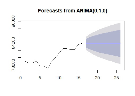
Modeling and Forecasting

Let’s now begin forecasting stock prices on the test dataset with a 95% confidence level.

# Forecast
fc, se, conf = fitted.forecast(321, alpha=0.05)  # 95% conf

# Make as pandas series
fc_series = pd.Series(fc, index=test_data.index)
lower_series = pd.Series(conf[:, 0], index=test_data.index)
upper_series = pd.Series(conf[:, 1], index=test_data.index)
# Plot
plt.figure(figsize=(10,5), dpi=100)
plt.plot(train_data, label='training data')
plt.plot(test_data, color = 'blue', label='Actual Stock Price')
plt.plot(fc_series, color = 'orange',label='Predicted Stock Price')
plt.fill_between(lower_series.index, lower_series, upper_series, 
                 color='k', alpha=.10)
plt.title('ARCH CAPITAL GROUP Stock Price Prediction')
plt.xlabel('Time')
plt.ylabel('ARCH CAPITAL GROUP Stock Price')
plt.legend(loc='upper left', fontsize=8)
plt.show()

Output:

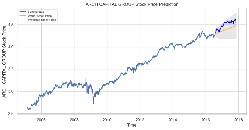
Evaluate Model Performance

Our model played great, as you can see. Let’s take a look at some of the most common accuracy metrics for evaluating forecast results:

# report performance
mse = mean_squared_error(test_data, fc)
print('MSE: '+str(mse))
mae = mean_absolute_error(test_data, fc)
print('MAE: '+str(mae))
rmse = math.sqrt(mean_squared_error(test_data, fc))
print('RMSE: '+str(rmse))
mape = np.mean(np.abs(fc - test_data)/np.abs(test_data))
print('MAPE: '+str(mape))

Output:

With a MAPE of around 2.5%, the model is 97.5% accurate in predicting the next 15 observations.

Also Read:

• Understand Random Forest Algorithms With Examples (Updated 2024)
• Guide to Sentiment Analysis using Natural Language Processing
• Guide on Support Vector Machine (SVM) Algorithm
• Understanding Sequential vs Functional API in Keras

Conclusion

Utilizing advanced learning techniques in Python provides a robust framework for stock market forecasting using the ARIMA model. This approach effectively analyzes price data and predicts price changes with high accuracy. By incorporating data mining methods to manage extensive datasets, our model supports real-time operations, yielding insights into stock trends. The ability to accurately forecast future market movements enhances investment strategies and underscores the importance of sophisticated analytics in modern financial markets.

Key Takeaways

• ARIMA models are powerful for forecasting stock market trends by analyzing historical data and identifying potential future price movements.
• The performance of the ARIMA model can be evaluated using metrics like MSE, MAE, RMSE, and MAPE, ensuring high accuracy in stock price predictions.
• The effectiveness of ARIMA models in predicting short-term market movements supports their use in developing informed trading strategies, thereby reducing investment risks.

Frequently Asked Questions

The media shown in this article are not owned by Analytics Vidhya and are used at the Author’s discretion.

Hardikkumar Dhaduk 31 May 2024