End to End Statistics for Data Science

Introduction

In the realm of data science, statistics play a pivotal role in data analysis and decision-making. As data scientists navigate through vast amounts of big data, they rely on both descriptive statistics and Bayesian methods to make sense of complex datasets. The use of tools like Excel for data visualization aids in presenting data in a comprehensible manner. In computer science, linear models and other statistical techniques are fundamental for interpreting data patterns and making informed decisions. Understanding and leveraging statistics is essential for extracting meaningful insights from data and driving effective strategies in any field.

Learning Outcomes

• Develop the skills to analyze and interpret complex datasets, making data-driven decisions as a proficient data analyst.
• Gain expertise in SQL, enabling efficient data extraction, manipulation, and management of large-scale databases.
• Grasp the fundamental concepts of linear algebra, crucial for advanced data analytics and machine learning methodologies.
• Learn to apply linear regression techniques to model relationships within statistical data, enhancing predictive analytics capabilities.
• Understand and implement various data analytics methodologies, ensuring robust and accurate data analysis.
• Explore the integration of artificial intelligence in data analytics, leveraging AI to uncover deeper insights and automate data-driven tasks.
• Master the techniques for analyzing statistical data, transforming raw data into actionable insights.

Importance of Statistics

• Using various statistical tests, determine the relevance of features.
• To avoid the risk of duplicate features, find the relationship between features.
• Putting the features into the proper format.
• Data normalization and scaling This step also entails determining the distribution of data as well as the nature of data.
• Taking the data for further processing and making the necessary modifications.
• Determine the best mathematical approach/model after processing the data.
• After the data are acquired, they are checked against the various accuracy measuring scales.

Acknowledge the Different Types of Analytics in Statistics

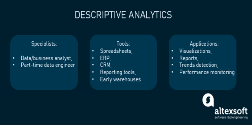
Descriptive Analytics

Descriptive analytics provides a retrospective view, answering the question, “What happened?” It helps businesses understand past performance by analyzing historical data and presenting it in a context that stakeholders can easily interpret. This foundational level of analytics is essential for identifying patterns within the data, and it is commonly associated with traditional business intelligence. Common visualizations used in descriptive analytics include pie charts, bar charts, tables, and line graphs, which help illustrate these patterns clearly.

Descriptive analytics is where every organization’s analytics journey should begin. By examining past events and identifying trends, businesses can gain valuable insights into their operations. This type of exploratory data analysis sets the stage for more advanced analytics by providing the necessary context for understanding data patterns. For example, analyzing sales data from the previous quarter can reveal whether sales increased or decreased, offering critical information for strategic decision-making in fields like cybersecurity, data engineering, and deep learning. By mastering descriptive analytics, one can effectively build the skills needed to progress into learning statistics and developing advanced learning algorithms.

Diagnostic Analytics

Diagnostic analytics delves deeper than descriptive analytics, helping you understand why something occurred in the past. This advanced form of analytics examines data or content to answer the question, “Why did it happen?” Techniques such as drill-down, data discovery, data processing, and correlation analysis are employed in this stage.

As the second step in the analytics process, diagnostic analytics builds on the insights gained from exploratory data analysis. Once an organization has established a clear picture of what happened, diagnostic analytics is applied to uncover the underlying reasons. This approach is particularly valuable in fields like cybersecurity, data engineering, and deep learning. By leveraging learning algorithms, learning statistics, and Python programming, organizations can gain a deeper understanding of their data and make informed decisions based on these insights.

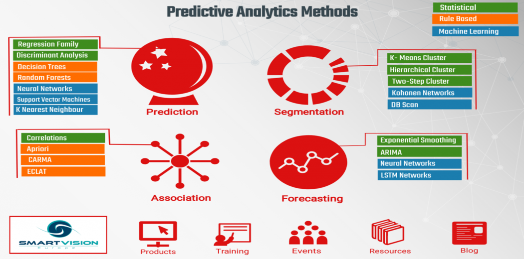
Predictive Analytics

Predictive analytics forecasts what is likely to happen in the future, providing businesses with data-driven, actionable insights. Once an organization has a firm grasp on what happened (descriptive analytics) and why it happened (diagnostic analytics), it can advance to predictive analytics. This advanced form of analytics seeks to answer the question, “What is likely to happen?” by utilizing data and knowledge.

The transition from diagnostic to predictive analytics is critical. Techniques such as multivariate analysis, forecasting, multivariate statistics, pattern matching, and predictive modeling are essential components of predictive analytics. Implementing these techniques can be challenging for organizations because they require large amounts of high-quality data and a thorough understanding of statistics and programming languages like R and Python.

Many organizations may lack the internal expertise needed to effectively implement a predictive model. However, the potential value of predictive analytics is enormous. For example, a predictive model can use historical data to forecast the impact of an upcoming marketing campaign on customer engagement. By accurately identifying which actions lead to specific outcomes, a company can predict which future actions will achieve the desired results. These insights are crucial for moving forward in the analytics journey.

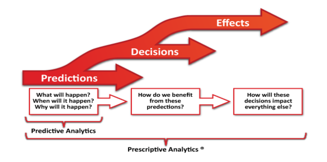
Prescriptive Analytics

Prescriptive analytics makes recommendations for actions that will capitalize on predictions and guide potential actions toward solutions. As the final and most advanced level of analytics, prescriptive analytics seeks to answer the question, “What should be done?” Techniques used in this type of analytics include graph analysis, simulation, complex event processing, neural networks, recommendation engines, heuristics, and machine learning.

Reaching this level of analytics is challenging. The accuracy of descriptive, diagnostic, and predictive analytics significantly impacts the reliability of prescriptive analytics. Achieving effective responses from prescriptive analysis requires high-quality data, a suitable data architecture, and expertise in implementing this architecture. Despite these challenges, the value of prescriptive analytics is immense, enabling organizations to make decisions based on thoroughly analyzed data rather than instinct, thereby increasing the likelihood of achieving desired outcomes, such as higher revenue. For example, in marketing, prescriptive analytics can help determine the optimal mix of channel engagement, such as identifying which customer segment is best reached via email.

Probability

In a Random Experiment, the probability is a measure of the likelihood that an event will occur. The number of favorable outcomes in an experiment with n outcomes is denoted by x. The following is the formula for calculating the probability of an event.

Probability (Event) = Favourable Outcomes/Total Outcomes = x/n

Let’s look at a simple application to better understand probability. If we need to know if it’s raining or not. There are two possible answers to this question: “Yes” or “No.” It is possible that it will rain or not rain. In this case, we can make use of probability. The concept of probability is used to forecast the outcomes of coin tosses, dice rolls, and card draws from a deck of playing cards.

Properties of Statistics 

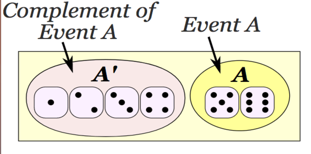
Complement

Ac, the complement of an event A in a sample space S, is the collection of all outcomes in S that are not members of set A. It is equivalent to rejecting any verbal description of event A.

P(A) + P(A’) = 1

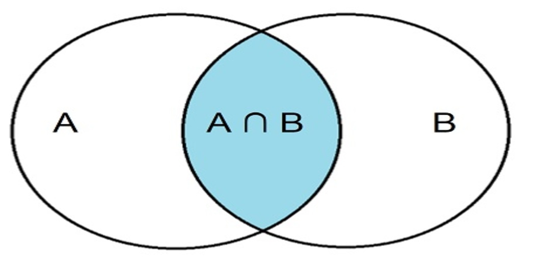
Intersection

The intersection of events is a collection of all outcomes that are components of both sets A and B. It is equivalent to combining descriptions of the two events with the word “and.”

P(A∩B) = P(A)P(B)

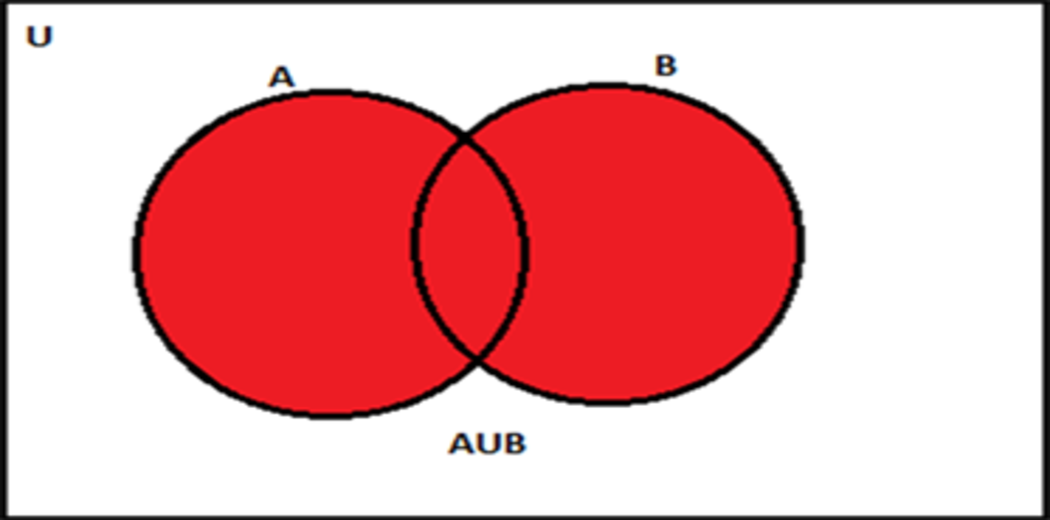
Union

The union of events is the collection of all outcomes that are members of one or both sets A and B. It is equivalent to combining descriptions of the two events with the word “or.”

P(A∪B) = P(A) + P(B) − P(A∩B)

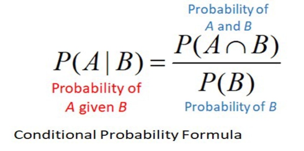
Conditional Probability

P(A|B) is a measure of the likelihood of one event happening in relation to one or more other events. When P(B)>0, P(A|B)=P(A|B)/P(B).

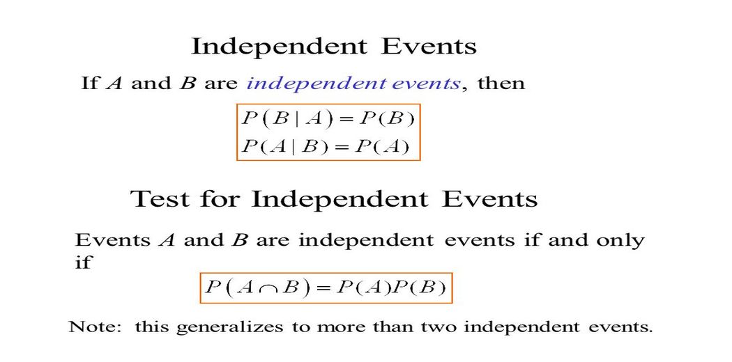
Independent Events

Two events are considered independent if the occurrence of one has no effect on the likelihood of the occurrence of the other. P(A|B)=P(A)P(B), where P(A)!= 0 and P(B)!= 0, P(A|B)=P(A), P(B|A)=P(A), P(A|B)=P(A), P(A|B)=P(A), P(B|A)=P(A), P(B|A)=P(A), P(B|A)=P(A), P( (B)

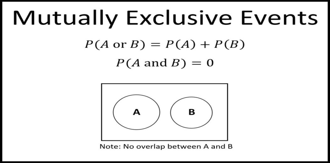
Mutually Exclusive Events

If events A and B share no elements, they are mutually exclusive. Because A and B have no outcomes in common, it is impossible for both A and B to occur on a single trial of the random experiment. This results in the following rule

P(A∩B) = 0

Any event A and its complement Ac are mutually exclusive if and only if A and B are mutually exclusive, but A and B can be mutually exclusive without being complements.

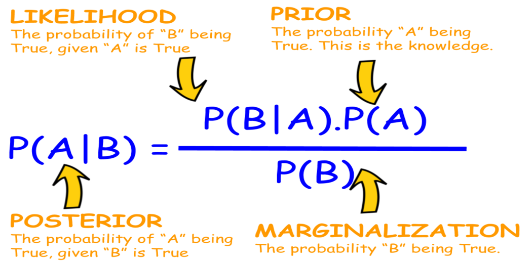
Bayes’ Theorem

It is a method for calculating conditional probability. The probability of an event occurring if it is related to one or more other events is known as conditional probability. For example, your chances of finding a parking space are affected by the time of day you park, where you park, and what conventions are taking place at any given time.

Central Tendency in Statistics

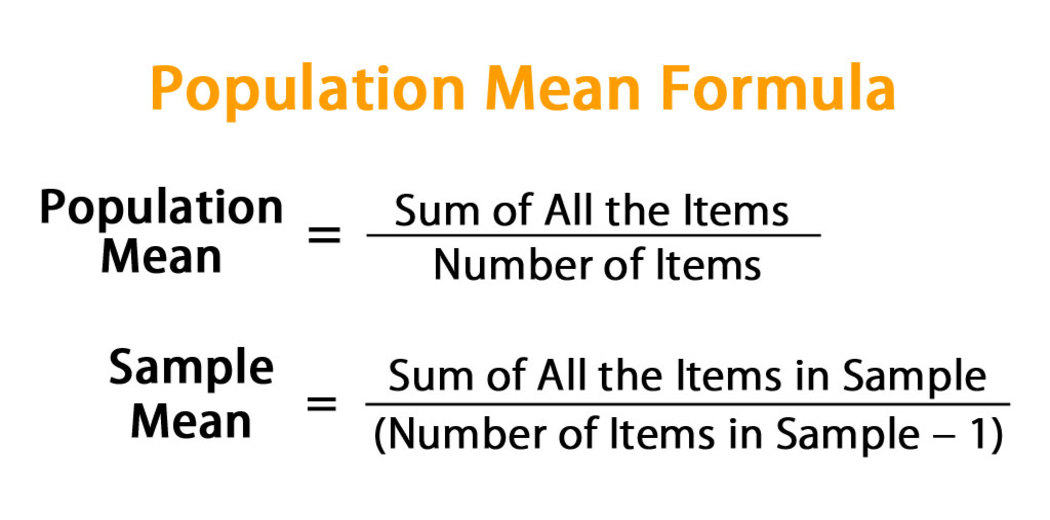
Mean

The mean (or average) is that the most generally used and well-known measure of central tendency. It will be used with both discrete and continuous data, though it’s most typically used with continuous data (see our styles of Variable guide for data types). The mean is adequate the sum of all the values within the data set divided by the number of values within the data set. So, if we have n values in a data set and they have values x1,x2, …,xn, the sample mean, usually denoted by “x bar”, is:

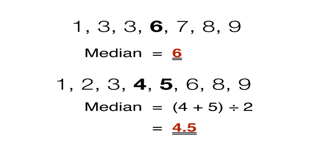
Median

The median value of a dataset is the value in the middle of the dataset when it is arranged in ascending or descending order. When the dataset has an even number of values, the median value can be calculated by taking the mean of the middle two values.

The following image gives an example for finding the median for odd and even numbers of samples in the dataset.

Mode

The mode is the value that appears the most frequently in your data set. The mode is the highest bar in a bar chart. A multimodal distribution exists when the data contains multiple values that are tied for the most frequently occurring. If no value repeats, the data does not have a mode.

Skewness

Skewness is a metric for symmetry, or more specifically, the lack of it. If a distribution, or data collection, looks the same to the left and right of the centre point, it is said to be symmetric.

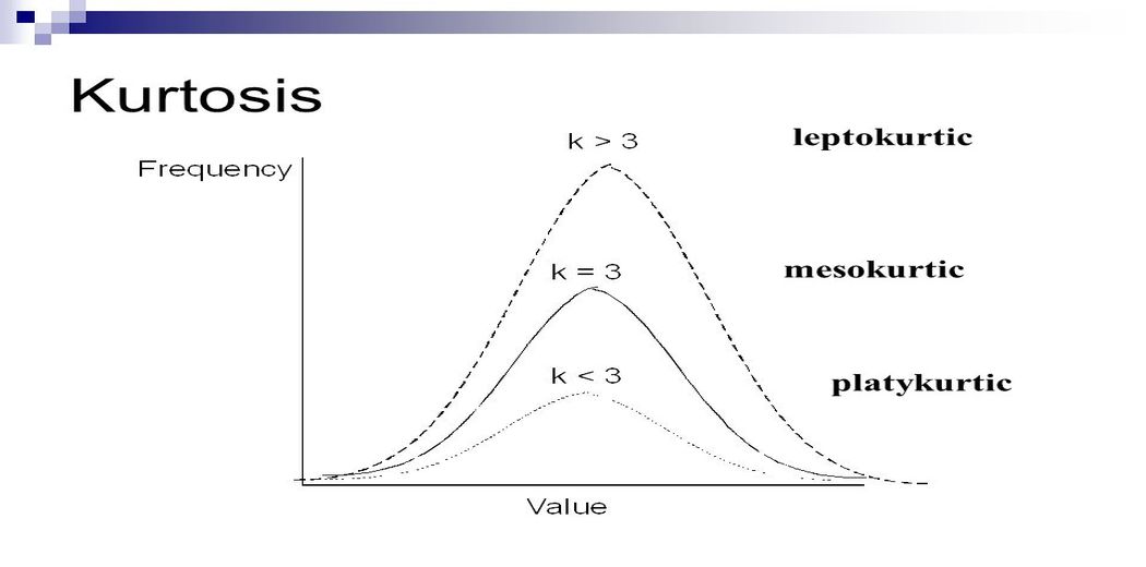
Kurtosis

Kurtosis is a measure of how heavy-tailed or light-tailed the data are in comparison to a normal distribution. Data sets having a high kurtosis are more likely to contain heavy tails or outliers. Light tails or a lack of outliers are common in data sets with low kurtosis.

Variability in Statistics

Range

In statistics, the range is the smallest of all dispersion measures. It is the difference between the distribution’s two extreme conclusions. In other words, the range is the difference between the distribution’s maximum and minimum observations.

Range = Xmax – Xmin

Where Xmax represents the largest observation and Xmin represents the smallest observation of the variable values.

Percentiles, Quartiles and Interquartile Range (IQR)

Percentiles: It is a statistician’s unit of measurement that indicates the value below which a given percentage of observations in a group of observations fall.

For instance, the value QX represents the 40th percentile of XX (0.40)

Quantiles: Values that divide the number of data points into four more or less equal parts, or quarters. Quantiles are the 0th, 25th, 50th, 75th, and 100th percentile values or the 0th, 25th, 50th, 75th, and 100th percentile values.

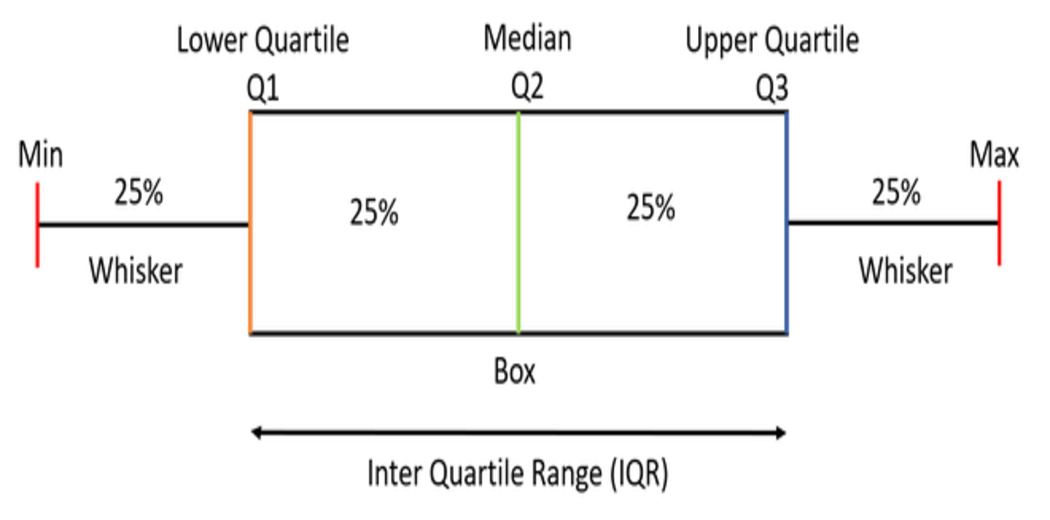
Interquartile Range (IQR): The difference between the third and first quartiles is defined by the interquartile range. The partitioned values that divide the entire series into four equal parts are known as quartiles. So, there are three quartiles. The first quartile, known as the lower quartile, is denoted by Q1, the second quartile by Q2, and the third quartile by Q3, known as the upper quartile. As a result, the interquartile range equals the upper quartile minus the lower quartile.

IQR = Upper Quartile – Lower Quartile

= Q3 − Q1

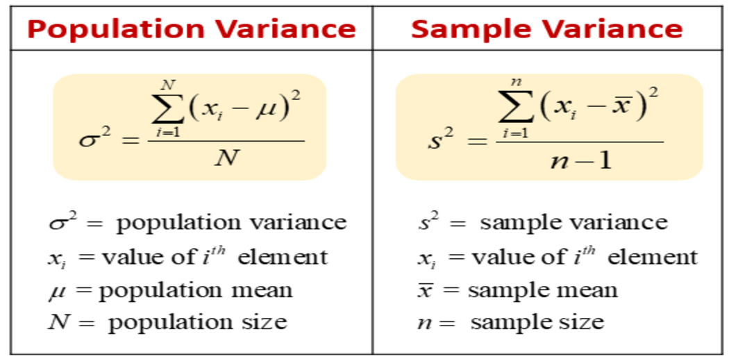
Variance

The dispersion of a data collection is measured by variance. It is defined technically as the average of squared deviations from the mean.

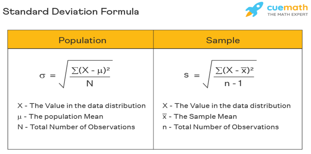
Standard Deviation

The standard deviation is a measure of data dispersion WITHIN a single sample selected from the study population. The square root of the variance is used to compute it. It simply indicates how distant the individual values in a sample are from the mean. To put it another way, how dispersed is the data from the sample? As a result, it is a sample statistic.

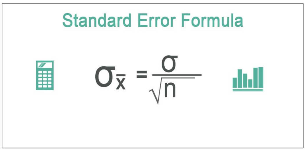
Standard Error (SE)

The standard error indicates how close the mean of any given sample from that population is to the true population mean. When the standard error rises, implying that the means are more dispersed, it becomes more likely that any given mean is an inaccurate representation of the true population mean. When the sample size is increased, the standard error decreases – as the sample size approaches the true population size, the sample means cluster more and more around the true population mean.

Relationship Between Variables

Causality: The term “causation” refers to a relationship between two events in which one is influenced by the other. There is causality in statistics when the value of one event, or variable, grows or decreases as a result of other events.

Each of the events we just observed may be thought of as a variable, and as the number of hours worked grows, so does the amount of money earned. On the other hand, if you work fewer hours, you will earn less money.

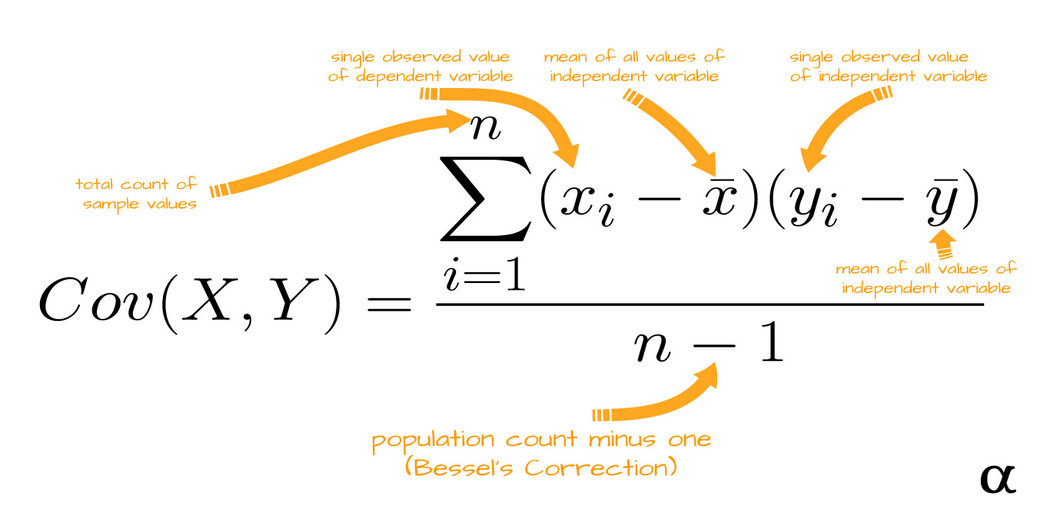
Covariance: Covariance is a measure of the relationship between two random variables in mathematics and statistics. The statistic assesses how much – and how far – the variables change in tandem. To put it another way, it’s a measure of the variance between two variables. The metric, on the other hand, does not consider the interdependence of factors. Any positive or negative value can be used for the variance.

The following is how the values are interpreted:

Positive covariance: When two variables move in the same direction, this is called positive covariance.

Negative covariance: It indicates that two variables are moving in opposite directions.

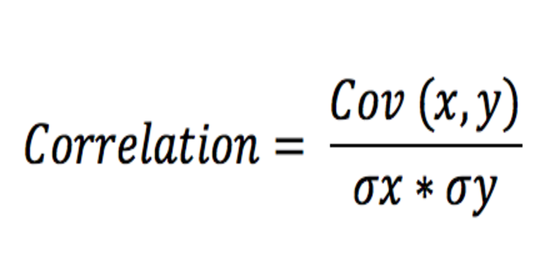
Correlation: Correlation is a statistical method for determining whether or not two quantitative or categorical variables are related. To put it another way, it’s a measure of how things are connected. Correlation analysis is the study of how variables are connected.

Here are a few examples of data with a high correlation:

• Your calorie consumption and weight.
• Your eye colour and the eye colours of your relatives.
• The amount of time you spend studying and your grade point average

Here are some examples of data with poor (or no) correlation:

• Your sexual preference and the cereal you eat are two factors to consider.
• The name of a dog and the type of dog biscuit that they prefer.
• The expense of vehicle washes and the time it takes to get a Coke at the station.

Correlations are useful because they allow you to forecast future behaviour by determining what relationship variables exist. In the social sciences, such as government and healthcare, knowing what the future holds is critical. Budgets and company plans are also based on these facts.

Probability Distributions

Probability Distribution Functions

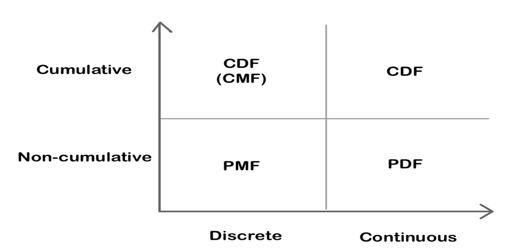
• Probability Mass Function (PMF): The probability distribution of a discrete random variable is described by the PMF, which is a statistical term. The terms PDF and PMF are frequently misunderstood. The PDF is for continuous random variables, whereas the PMF is for discrete random variables. Throwing a dice, for example (you can only choose from 1 to 6 numbers (countable))
• Probability Density Function (PDF): The probability distribution of a continuous random variable is described by the word PDF, which is a statistical term. The Gaussian Distribution is the most common distribution used in PDF. If the features / random variables are Gaussian distributed, then the PDF will be as well. Because the single point represents a line that does not span the area under the curve, the probability of a single outcome is always 0 on a PDF graph.
• Cumulative Density Function (CDF): The cumulative distribution function can be used to describe the continuous or discrete distribution of random variables.

If X is the height of a person chosen at random, then F(x) is the probability of the individual being shorter than x. If F(180 cm)=0.8, then an individual chosen at random has an 80% chance of being shorter than 180 cm (equivalently, a 20 per cent chance that they will be taller than 180cm).

Continuous Probability Distribution

• Uniform Distribution: Uniform distribution is a sort of probability distribution in statistics in which all events are equally likely. Because the chances of drawing a heart, a club, a diamond, or a spade are equal, a deck of cards contains uniform distributions. Because the likelihood of receiving heads or tails in a coin toss is the same, a coin has a uniform distribution.

A coin flip that returns a head or tail has a probability of p = 0.50 and would be represented by a line from the y-axis at 0.50.

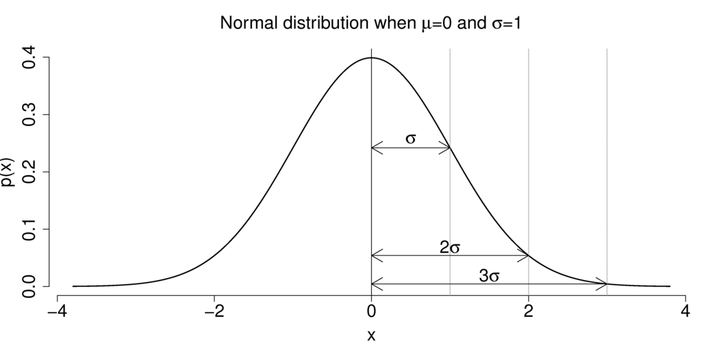
• Normal/Gaussian Distribution: The normal distribution, also known as the Gaussian distribution, is a symmetric probability distribution centred on the mean, indicating that data around the mean occur more frequently than data far from it. The normal distribution will show as a bell curve on a graph.

Points to remember:

A probability bell curve is referred to as a normal distribution. The mean of a normal distribution is 0 and the standard deviation is 1. It has a kurtosis of 3 and zero skew. Although all symmetrical distributions are normal, not all normal distributions are symmetrical. Most pricing distributions aren’t totally typical.

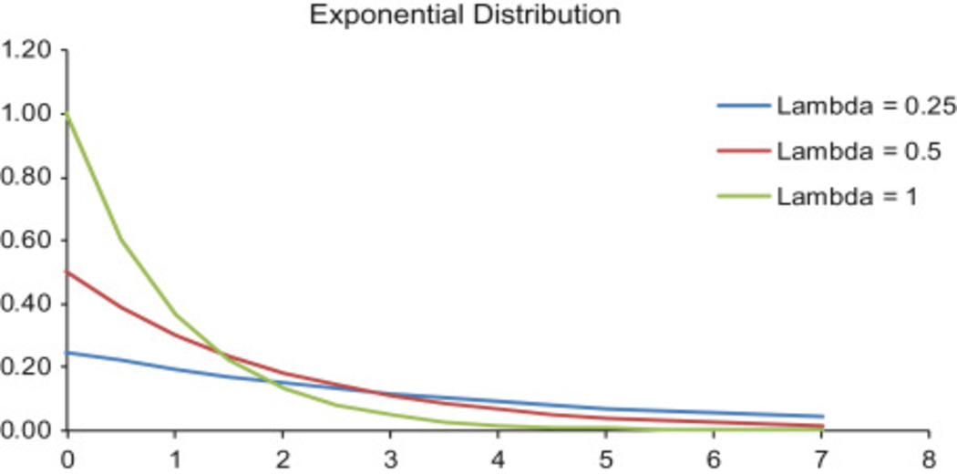
• Exponential Distribution: The exponential distribution is a continuous distribution used to estimate the time it will take for an event to occur. For example, in physics, it is frequently used to calculate radioactive decay, in engineering, it is frequently used to calculate the time required to receive a defective part on an assembly line, and in finance, it is frequently used to calculate the likelihood of a portfolio of financial assets defaulting. It can also be used to estimate the likelihood of a certain number of defaults occurring within a certain time frame.

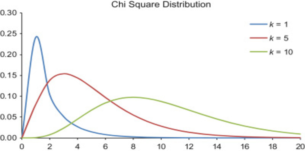
• Chi-Square Distribution: A continuous distribution with degrees of freedom is called a chi-square distribution. It’s used to describe a sum of squared random variable’s distribution. It’s also used to determine whether a data distribution’s goodness of fit is good, whether data series are independent, and to estimate confidence intervals around variance and standard deviation for a random variable from a normal distribution. Furthermore, the chi-square distribution is a subset of the gamma distribution.

Discrete Probability Distribution

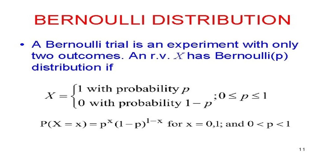
• Bernoulli Distribution: A Bernoulli distribution is a discrete probability distribution for a Bernoulli trial, which is a random experiment with just two outcomes (named “Success” or “Failure” in most cases). When flipping a coin, the likelihood of getting ahead (a “success”) is 0.5. “Failure” has a chance of 1 – P. (where p is the probability of success, which also equals 0.5 for a coin toss). For n = 1, it is a particular case of the binomial distribution. In other words, it’s a single-trial binomial distribution (e.g. a single coin toss).

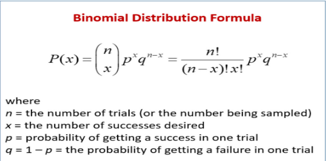
• Binomial Distribution: A discrete distribution is a binomial distribution. It’s a well-known probability distribution. The model is then used to depict a variety of discrete phenomena seen in business, social science, natural science, and medical research.

Because of its relationship with a binomial distribution, the binomial distribution is commonly employed. For binomial distribution to be used,

The following conditions must be met:

• There are n identical trials in the experiment, with n being a limited number.
• Each trial has only two possible outcomes, i.e., each trial is a Bernoulli’s trial.
• One outcome is denoted by the letter S (for success) and the other by the letter F (for failure) (for failure).
• From trial to trial, the chance of S remains the same. The chance of success is represented by p, and the likelihood of failure is represented by q (where p+q=1).
• Each trial is conducted independently.
• The number of successful trials in n trials is the binomial random variable x.

If X reflects the number of successful trials in n trials under the preceding conditions, then x is said to follow a binomial distribution with parameters n and p.

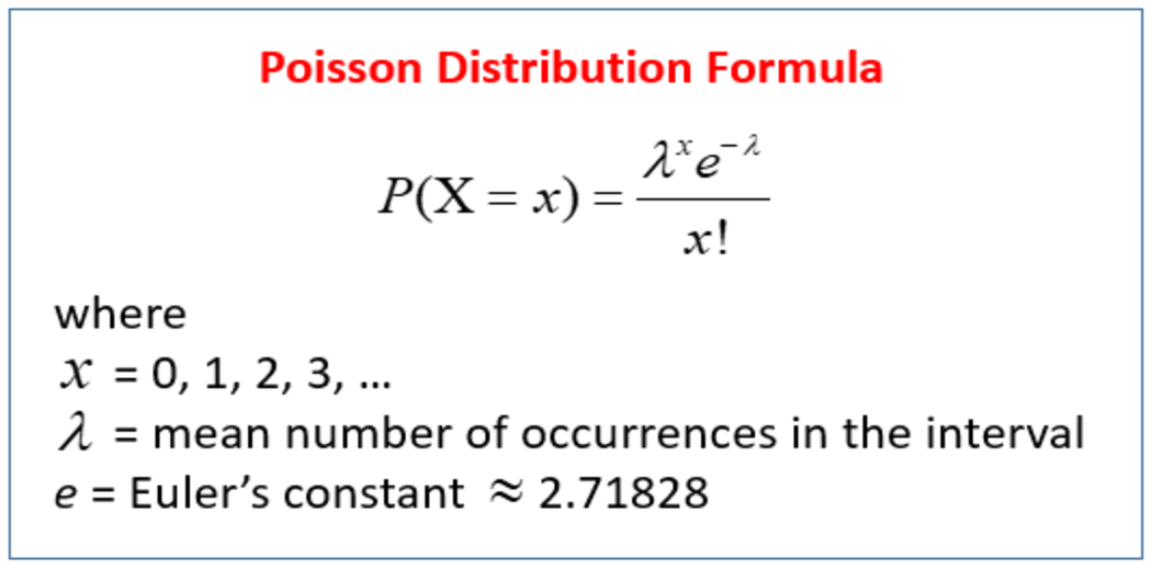
• Poisson Distribution: A Poisson distribution is a probability distribution used in statistics to show how many times an event is expected to happen over a certain amount of time. To put it another way, it’s a count distribution. Poisson distributions are frequently accustomed comprehend independent events that occur at a gradual rate during a selected timeframe.

The Poisson distribution is a discrete function, which means the variable can only take values from a (possibly endless) list of possibilities. To put it another way, the variable can’t take all of the possible values in any continuous range. The variable can only take the values 0, 1, 2, 3, etc., with no fractions or decimals, in the Poisson distribution (a discrete distribution).

Hypothesis Testing and Statistical Significance in Statistics

Hypothesis testing may be a method within which an analyst verifies a hypothesis a couple of population parameters. The analyst’s approach is set by the kind of the info and also the purpose of the study. the utilization of sample data to assess the plausibility of a hypothesis is thought of as hypothesis testing.

Null and Alternative Hypothesis

Null Hypothesis (H0)

A population parameter (such as the mean, standard deviation, and so on) is equal to a hypothesised value, according to the null hypothesis. The null hypothesis is a claim that is frequently made based on previous research or specialised expertise.

Alternative hypothesis (H1)

The alternative hypothesis says that a population parameter is less, more, or different than the null hypothesis’s hypothesised value. The alternative hypothesis is what you believe or want to prove to be correct.

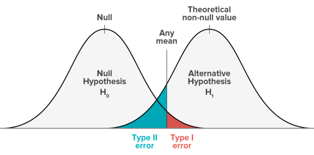
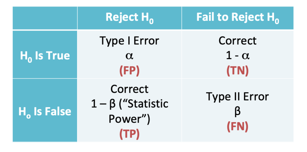
Type 1 and Type 2 error

Type 1 error

A type 1 error, often referred to as a false positive, happens when a researcher rejects a real null hypothesis incorrectly. this suggests you’re claiming your findings are noteworthy after they actually happened by coincidence.

Your alpha level (), which is that the p-value below which you reject the null hypothesis, represents the likelihood of constructing a sort I error. When rejecting the null hypothesis, a p-value of 0.05 indicates a 5% chance of being mistaken.

By setting p to a lesser value, you’ll lessen your chances of constructing a kind I error.

Type 2 error

A type II error, commonly referred to as a false negative, occurs when a researcher fails to reject a null hypothesis that is actually true. In this case, the researcher concludes that there is no significant influence, when in fact there is.

Beta () is that the probability of creating a sort II error, and it’s proportional to the statistical test’s power (power = 1- ). By ensuring that your test has enough power, you’ll reduce your chances of constructing a sort II error.

This can be accomplished by ensuring that your sample size is sufficient to spot a practical difference when one exists.

Interpretation

P-value

The p-value in statistics is that the likelihood of getting outcomes a minimum of as extreme because the observed results of a statistical hypothesis test, given the null hypothesis is valid. The p-value, instead of rejection points, is employed to work out the smallest amount level of significance at which the null hypothesis is rejected. A lower p-value indicates that the choice hypothesis has more evidence supporting it.

Critical Value

It is a point on the test distribution that is compared to the test statistic to see if the null hypothesis should be rejected. Reject the null hypothesis if the absolute test statistic exceeds the critical value, indicating statistical significance.

Significance Level and Rejection Region

The probability that an event (such as a statistical test) occurred by chance is the significance level of the occurrence. We call an occurrence significant if the level is very low, i.e., the possibility of it happening by chance is very minimal. The rejection region depends on the significance level α, indicating the probability of Type I error. This significance level is a critical parameter in hypothesis testing.

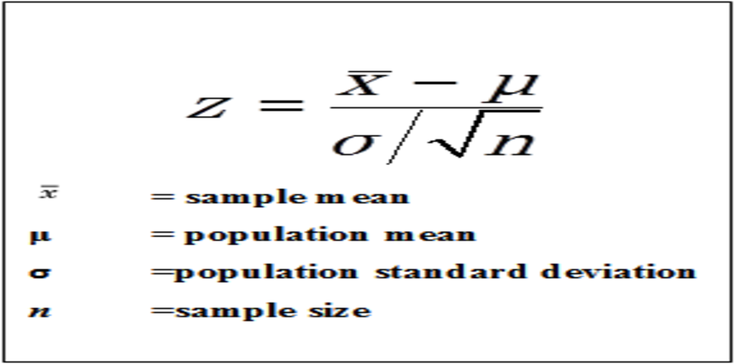
Z-Test

The z-test may be a hypothesis test within which the z-statistic is distributed normally. The z-test is best utilized for samples with quite 30 because, in line with the central limit theorem, samples with over 30 samples are assumed to be approximately regularly distributed.

The null and alternative hypotheses, also because the alpha and z-score, should all be reported when doing a z-test. The test statistic should next be calculated, followed by the results and conclusion. A z-statistic, also called a z-score, could be a number that indicates what number of standard deviations a score produced from a z-test is above or below the mean population.

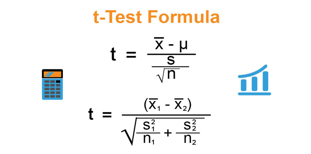
T-Test

A t-test is an inferential statistic that’s won’t see if there’s a major difference within the means of two groups that are related in how. It’s most ordinarily employed when data sets, like those obtained by flipping a coin 100 times, are expected to follow a traditional distribution and have unknown variances. A t-test could be a hypothesis-testing technique that will be accustomed to assess an assumption that’s applicable to a population.

ANOVA (Analysis of Variance)

ANOVA is the way to find out if experimental results are significant. One-way ANOVA compares two means from two independent groups using only one independent variable. Two-way ANOVA is the extension of one-way ANOVA using two independent variables to calculate the main effect and interaction effect.

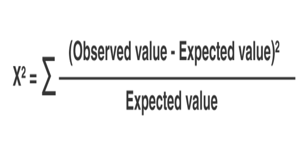
Chi-Square Test

It is a test that assesses how well a model matches actual data. A chi-square statistic requires data that is random, raw, mutually exclusive, and collected from independent variables. Additionally, the data must be drawn from a sufficiently large sample. The outcomes of a fair coin flip, for example, meet these conditions.

In hypothesis testing, chi-square tests are frequently utilized. The chi-square statistic examines disparities between expected and actual results given sample size and variables.

Conclusion

Understanding key statistical concepts and probability theory is crucial for anyone pursuing a data science course. These foundational elements enable you to perform accurate data analysis and make informed decisions based on data insights. By mastering statistics and probability, you’ll be well-equipped to navigate through various levels of analytics—from descriptive and diagnostic to predictive and prescriptive. As you delve deeper into data science, these skills will enhance your ability to extract meaningful patterns from data and forecast future trends. By developing actionable recommendations, you will ultimately drive success in your analytics journey.

The media shown in this article is not owned by Analytics Vidhya and are used at the Author’s discretion

Gunjan Agarwal 29 May 2024

I am Data Science Fresher. And I'm open to work.