Introduction

Regression is a fundamental technique in machine learning used to analyze relationships between variables and make predictions. This article explores the basics of regression, focusing on linear regression, its implementation using gradient descent, and its practical application. Understanding these concepts is essential for anyone looking to delve into predictive modeling and data analysis.

Learning Outcomes

• Learn how regression models find correlations between variables, supporting predictive analysis.
• Explore different types such as linear, polynomial, and logistic regression, each suited to specific data characteristics.
• Grasp the fundamentals of simple and multiple linear regression, including the slope-intercept form.
• Understand gradient descent’s role in optimizing linear regression models by minimizing the mean squared error.
• Discover how the learning rate affects the convergence and performance of gradient descent.
• Implement linear regression in Python, from dataset definition to model evaluation, using mean squared error.

This article was published as a part of the Data Science Blogathon.

What is a Regression?

In Regression, we plot a graph between the variables which best fit the given data points. The machine learning model can deliver predictions regarding the data. In naïve words, “Regression shows a line or curve that passes through all the data points on a target-predictor graph in such a way that the vertical distance between the data points and the regression line is minimum.” It is used principally for prediction, forecasting, time series modeling, and determining the causal-effect relationship between variables.

Application Areas

People widely use regression in:

• Prediction: Estimating future values based on historical data.
• Forecasting: Predicting trends over time.
• Causal Relationships: Determining how changes in one variable affect another.

Types of Regression Models

Let us now explore types of regression models:

• Linear Regression
• Polynomial Regression
• Logistics Regression

Linear Regression

Linear regression is a simple and commonly used regression model. It assumes a linear relationship between a dependent variable (Y-axis) and one or more independent variables (X-axis). The relationship is represented by the equation: Y = a + bX

• YYY is the dependent variable.
• XXX is the independent variable.
• aaa is the intercept (the value of YYY when X=0X = 0X=0).
• bbb is the slope of the line (the rate of change in YYY with respect to XXX).

Simple Linear Regression: When there’s only one independent variable, it’s called simple linear regression. For example, predicting house prices based on their area.

Multiple Linear Regression:

When there are multiple independent variables, we call it multiple linear regression. For example, predicting a person’s salary based on years of experience, education level, and location.

Polynomial Regression

Polynomial regression is a form of linear regression in which the relationship between the independent variable XXX and the dependent variable YYY is modeled as an nnn-th degree polynomial. It’s useful when the relationship between variables isn’t linear. The equation for polynomial regression is: Y=a0+a1X+a2X2+…+anXnY = a_0 + a_1X + a_2X^2 + … + a_nX^nY=a0​+a1​X+a2​X2+…+an​Xn where:

• a0,a1,…,ana_0, a_1, …, a_na0​,a1​,…,an​ are the coefficients to be determined.
• X2,X3,…,XnX^2, X^3, …, X^nX2,X3,…,Xn are the higher-order terms.

Logistic Regression

Despite its name, logistic regression is a statistical method used for binary classification, not regression. It estimates the probability that an instance belongs to a particular class (e.g., yes/no, 1/0). The predicted values are mapped to [0, 1] through the logistic function (sigmoid function): P(Y=1∣X)=11+e−(a+bX)P(Y=1|X) = \frac{1}{1 + e^{-(a + bX)}}P(Y=1∣X)=1+e−(a+bX)1​ where:

• P(Y=1∣X)P(Y=1|X)P(Y=1∣X) is the probability that the dependent variable YYY is 1 given the independent variable XXX.
• aaa is the intercept.
• bbb is the coefficient of the independent variable.

Logistic regression commonly finds application in various fields, including healthcare (predicting disease presence), finance (predicting default probability), and marketing (predicting customer churn).

What is Linear Regression?

Linear regression is a quiet and simple statistical regression method used for predictive analysis and shows the relationship between the continuous variables. Linear regression shows the linear relationship between the independent variable (X-axis) and the dependent variable (Y-axis), consequently called linear regression. If there is a single input variable (x), we call such linear regression simple linear regression. If there are more than one input variable, we call it multiple linear regression. The linear regression model gives a sloped straight line describing the relationship within the variables.

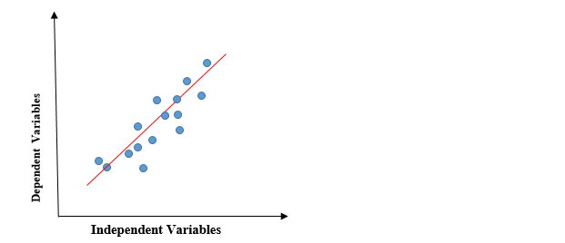
The above graph presents the linear relationship between the dependent variable and independent variables. When the value of x (independent variable) increases, the value of y (dependent variable) is likewise increasing. The red line is referred to as the best fit straight line. Based on the given data points, we try to plot a line that models the points the best.

To calculate best-fit line linear regression uses a traditional slope-intercept form.

• y= Dependent Variable.
• x= Independent Variable.
• a0= intercept of the line.
• a1 = Linear regression coefficient.

Need of a Linear regression

As mentioned above, Linear regression estimates the relationship between a dependent variable and an independent variable. Let’s understand this with an easy example:

Let’s say we want to estimate the salary of an employee based on year of experience. You have the recent company data, which indicates that the relationship between experience and salary. Here year of experience is an independent variable, and the salary of an employee is a dependent variable, as the salary of an employee is dependent on the experience of an employee. Using this insight, we can predict the future salary of the employee based on current & past information.

A regression line can be a Positive Linear Relationship or a Negative Linear Relationship.

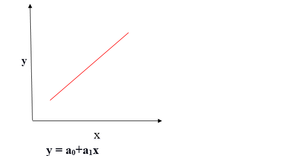
Positive Linear Relationship

If the dependent variable expands on the Y-axis and the independent variable progress on X-axis, then such a relationship is termed a Positive linear relationship.

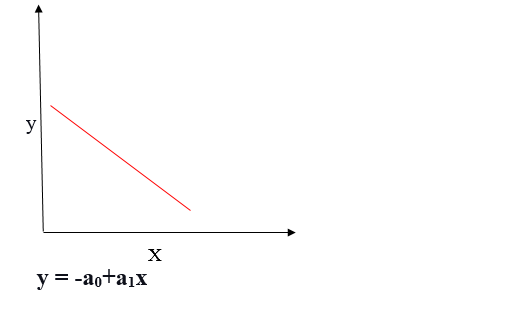
Negative Linear Relationship

If the dependent variable decreases on the Y-axis while the independent variable increases on the X-axis, we refer to this relationship as a negative linear relationship.

The goal of the linear regression algorithm is to get the best values for a0 and a1 to find the best fit line. The best fit line should minimize the error between predicted values and actual values, ensuring that the error is minimized.

What is Cost function?

The cost function helps to figure out the best possible values for a0 and a1, which provides the best fit line for the data points.

Cost function optimizes the regression coefficients or weights and measures how a linear regression model is performing. The cost function measures the accuracy of the mapping function that maps the input variable to the output variable. This mapping function is also known as the Hypothesis function.

In Linear Regression, we use the Mean Squared Error (MSE) cost function, which averages the squared errors between the predicted values and actual values.

By simple linear equation y=mx+b we can calculate MSE as:

Let’s y = actual values, y_i = predicted values

Using the MSE function, we will change the values of a0 and a1 such that the MSE value settles at the minima.

We can manipulate the model parameters a0a_0a0​ and a1a_1a1​ (xi, b) to minimize the cost function. We use the gradient descent method to determine these parameters so that we can minimize the cost function value.

What is Gradient descent ?

Gradient descent is a method of updating a0 and a1 to minimize the cost function (MSE). A regression model uses gradient descent to update the coefficients of the line (a0, a1 => xi, b) by reducing the cost function by a random selection of coefficient values and then iteratively update the values to reach the minimum cost function.

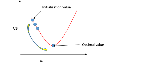
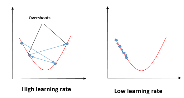
Imagine a pit in the shape of U. You are standing at the topmost point in the pit, and your objective is to reach the bottom of the pit. There is a treasure, and you can only take a discrete number of steps to reach the bottom. If you decide to take one footstep at a time, you would eventually get to the bottom of the pit but, this would take a longer time. If you choose to take longer steps each time, you may get to sooner but, there is a chance that you could overshoot the bottom of the pit and not near the bottom. In the gradient descent algorithm, the number of steps you take is the learning rate, and this decides how fast the algorithm converges to the minima.

To update a₀ and a₁, we take gradients from the cost function. To find these gradients, we take partial derivatives for a₀ and a₁.

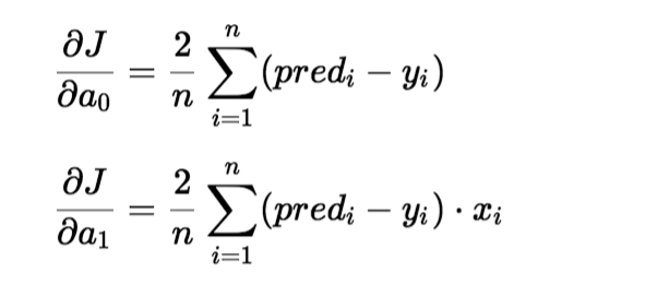
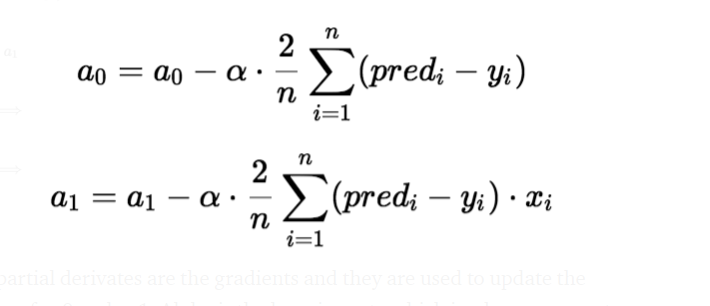
The gradients use the partial derivatives to update the values of a0 and a1. Alpha is the learning rate.

Impact of Different Values for Learning Rate

The blue line minimizes the cost function value in a few iterations, representing the optimal value of the learning rate. The green line represents if the learning rate is lower than the optimal value, then the number of iterations required high to minimize the cost function. If the learning rate selected is very high, the cost function could continue to increase with iterations and saturate at a value higher than the minimum value, that represented by a red and black line.

Steps to Implement Linear Regression Model

In this, I will take random numbers for the dependent variable (salary) and an independent variable (experience) and will predict the impact of a year of experience on salary.

Step1: Import Required Libraries

import matplotlib.pyplot as plt
import pandas as pd
import numpy as np

Step2: Define the Dataset

x= np.array([2.4,5.0,1.5,3.8,8.7,3.6,1.2,8.1,2.5,5,1.6,1.6,2.4,3.9,5.4])
y = np.array([2.1,4.7,1.7,3.6,8.7,3.2,1.0,8.0,2.4,6,1.1,1.3,2.4,3.9,4.8])
n = np.size(x)

Step3: Plot the Data Points

import matplotlib.pyplot as plt
import pandas as pd
import numpy as np

x= np.array([2.4,5.0,1.5,3.8,8.7,3.6,1.2,8.1,2.5,5,1.6,1.6,2.4,3.9,5.4])
y = np.array([2.1,4.7,1.7,3.6,8.7,3.2,1.0,8.0,2.4,6,1.1,1.3,2.4,3.9,4.8])
n = np.size(x)

plt.scatter(x, y, color = 'red')
plt.xlabel("Experience")
plt.ylabel("Salary")
plt.show()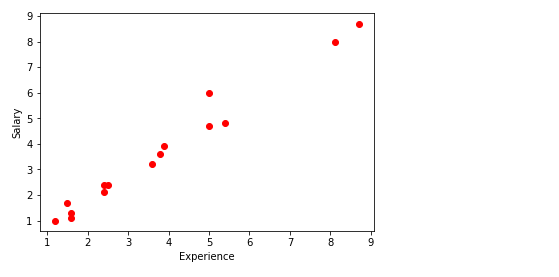

The main function to calculate values of coefficients

• Initialize the parameters.
• Predict the value of a dependent variable by given an independent variable.
• Calculate the error in prediction for all data points.
• Calculate partial derivative w.r.t a0 and a1.
• Calculate the cost for each number and add them.
• Update the values of a0 and a1.

#initialize the parameters
a0 = 0                  #intercept
a1 = 0                  #Slop
lr = 0.0001             #Learning rate
iterations = 1000       # Number of iterations
error = []              # Error array to calculate cost for each iterations.
for itr in range(iterations):
    error_cost = 0
    cost_a0 = 0
    cost_a1 = 0
    for i in range(len(experience)):
        y_pred = a0+a1*experience[i]   # predict value for given x
        error_cost = error_cost +(salary[i]-y_pred)**2
        for j in range(len(experience)):
            partial_wrt_a0 = -2 *(salary[j] - (a0 + a1*experience[j]))                #partial derivative w.r.t a0
            partial_wrt_a1 = (-2*experience[j])*(salary[j]-(a0 + a1*experience[j]))   #partial derivative w.r.t a1
            cost_a0 = cost_a0 + partial_wrt_a0      #calculate cost for each number and add
            cost_a1 = cost_a1 + partial_wrt_a1      #calculate cost for each number and add
        a0 = a0 - lr * cost_a0    #update a0
        a1 = a1 - lr * cost_a1    #update a1
        print(itr,a0,a1)          #Check iteration and updated a0 and a1
    error.append(error_cost)      #Append the data in array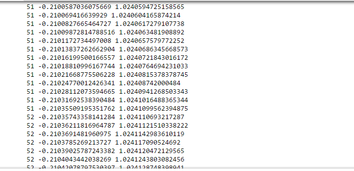

At approximate iteration 50- 60, we got the value of a0 and a1.

print(a0)
print(a1)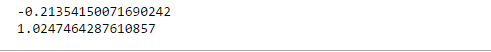

Step4: Plotting the Error for Each Iteration.

plt.figure(figsize=(10,5))
plt.plot(np.arange(1,len(error)+1),error,color='red',linewidth = 5)
plt.title("Iteration vr error")
plt.xlabel("iterations")
plt.ylabel("Error")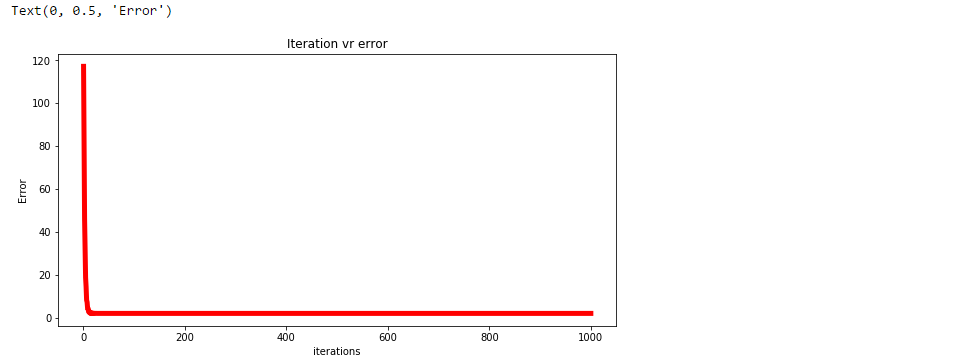

Step5: Predicting the Values

pred = a0+a1*experience
print(pred)

Step6: Plot the Regression Line

plt.scatter(experience,salary,color = 'red')
plt.plot(experience,pred, color = 'green')
plt.xlabel("experience")
plt.ylabel("salary")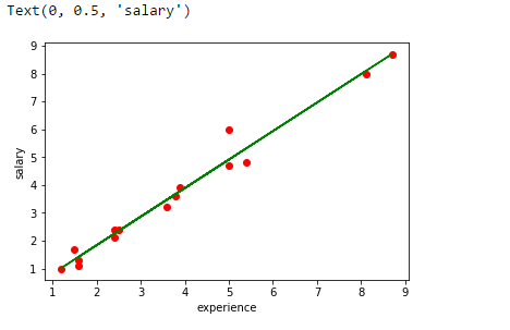

Step7: Analyze Performance of the Model by Calculating MSE

error1 = salary - pred
se = np.sum(error1 ** 2)
mse = se/n
print("mean squared error is", mse)

Step8: Use scikit Library to Confirm Above Steps

from sklearn.linear_model import LinearRegression
from sklearn.metrics import mean_squared_error 
experience = experience.reshape(-1,1)
model = LinearRegression()
model.fit(experience,salary)
salary_pred = model.predict(experience)
Mse = mean_squared_error(salary, salary_pred)
print('slop', model.coef_)
print("Intercept", model.intercept_)
print("MSE", Mse)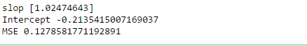

Conclusion

Regression analysis offers powerful tools for understanding and predicting relationships between variables. We explored three main types of regression models: Linear Regression, which depicts linear relationships; Polynomial Regression, suited for nonlinear data; and Logistic Regression, used for binary classification. Each model has unique applications across various fields, from predicting sales trends in business to analyzing medical data. Mastering these regression techniques equips data scientists with essential skills to uncover insights and make informed decisions in diverse domains.

Key Takeaways

• Regression models help understand and predict relationships between variables, making them essential tools in data science.
• Ideal for modeling linear relationships between variables, commonly used in predictive analytics.
• Suitable for non-linear relationships, it provides flexibility in modeling complex data patterns.
• Despite its name, used for classification tasks, estimating probabilities of class membership.
• Regression models find applications in diverse fields like finance, healthcare, and marketing for predicting trends, forecasting, and identifying causal relationships.
• Mastering these regression techniques equips data scientists with essential skills to derive insights and make data-driven decisions across various domains.

Frequently Asked Questions

The media shown in this article are not owned by Analytics Vidhya and are used at the Author’s discretion.