Introduction to Classification Problem using PySpark
This article was published as a part of the Data Science Blogathon.
Introduction
We are keeping forward with the PySpark series, where by far, we covered Data preprocessing techniques and various ML algorithms along with real-world consulting projects. In this article as well, we will work on another consulting project. Let’s take a scenario, Suppose a Dog Food company has hired us, and our task is to predict why their manufactured food is being spoiled rapidly compared to their shelf’s life. We will solve this particular problem statement using PySpark’s MLIB.
About the Problem statement
From the introduction part, we are well aware of “what” needs to be done, but in this section, we will dig more to understand the “how” and “why” parts of this project.
Why Does Dog Food company need us?
- From the last few supply chain tenure, they are regularly facing the pre-spoiling of the dog food, and they have figured out the reason as well, as they have not upgraded to the latest machinery, so the four secret ingredients are not mixing up well. But they cannot figure out among those 4 chemicals which one is responsible or has the strongest effect.
How are we gonna approach this problem statement?
- Our main task is to predict that 1 chemical/preservative has the strongest effect among those 4 ingredients, and to achieve this, we are not gonna follow the train test split methodology but instead feature importance method because, in the end, that only will let us know which of those ingredients is most responsible for spoiling the dog food before its shelf life.
About the dataset
This dataset holds 4 feature columns labeled B, C, and D, and the other Target column is labeled “Spoiled.” So a total of 5 columns are there in the dataset. Let’s look at the short description of each column.
- Preservative_A: Percentage of A ingredient in the mixture.
- Preservative_B: Percentage of B ingredient in the mixture.
- Preservative_C: Percentage of C ingredient in the mixture.
- Preservative_D: Percentage of D ingredient in the mixture.
Here you can find the source of the dataset.
Note: In this particular project, we will not follow that generalized method of machine learning pipeline (train-test-split); instead, we will go with another method which you will find out while moving on with this article, which will help you to draw another template for such problems.
Installing PySpark: To do the predictive analysis on the spoiling chemical, we just need to install one library, which is the heart and soul of this project, i.e., PySpark, that will eventually set up an environment for the MLIB library and establish a connection with Apache Spark.
Spark Session
In this part of the article, we will start the Spark Session because this is one of those mandatory processes where we set up the environment with apache Spark by creating and new session via PySpark.
from pyspark.sql import SparkSession
spark = SparkSession.builder.appName('dog_food_project').getOrCreate()
spark
Output:
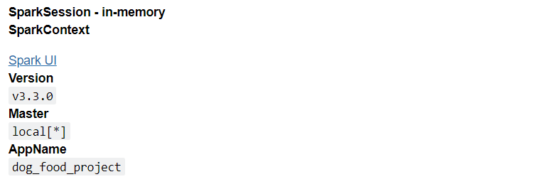
Inference: First and foremost, the Spark Session library is imported from the pyspark.sql library.
Then comes the role of the builder function that will build the session (providing that naming functionality too – dog_food_project) after building it, we created the SparkSession using the getOrCreate() function.
At the last call the spark object, we can see the UI of the SparkMemory that summarizes the whole process.
Reading the Dog Food Dataset with PySpark
Here is yet another compulsory step to be followed because any data science project is impossible to carry on without the relevant dataset it’s like “trying to build the house without considering bricks“. Hence one can refer to the below code to read the dataset, which is in the CSV format.
data_food = spark.read.csv('dog_food.csv',inferSchema=True,header=True)
data_food.show()
Output:
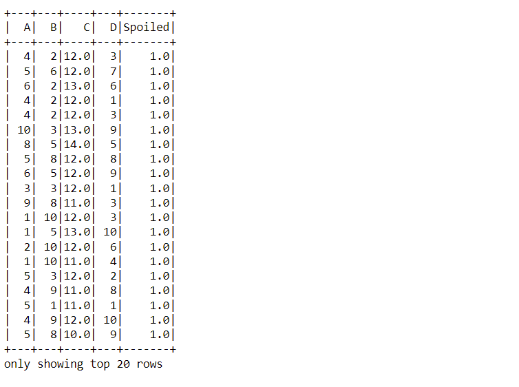
Inference: From the above output we have confirmed what we stated regarding the dataset in the About section i.e. it has 4 ingredients/chemicals (A, B, C, D) and one target variable i.e. Spoiled.
For doing so, the read.csv function was used, keeping the inferSchema and header parameter as True so that it can return the relevant type of data.
data_food.printSchema()
Output:
root
 |-- A: integer (nullable = true)
 |-- B: integer (nullable = true)
 |-- C: double (nullable = true)
 |-- D: integer (nullable = true)
 |-- Spoiled: double (nullable = true)
Inference: Just before this step, while reading the dataset, we put the inferSchema parameter value to True so that while performing the printSchema function, we can get the right data type for each feature. Hence all 4 feature has the integer type and Spoiled (target) holds the double type of data.
data_food.head(10)
Output:
[Row(A=4, B=2, C=12.0, D=3, Spoiled=1.0),
 Row(A=5, B=6, C=12.0, D=7, Spoiled=1.0),
 Row(A=6, B=2, C=13.0, D=6, Spoiled=1.0),
 Row(A=4, B=2, C=12.0, D=1, Spoiled=1.0),
 Row(A=4, B=2, C=12.0, D=3, Spoiled=1.0),
 Row(A=10, B=3, C=13.0, D=9, Spoiled=1.0),
 Row(A=8, B=5, C=14.0, D=5, Spoiled=1.0),
 Row(A=5, B=8, C=12.0, D=8, Spoiled=1.0),
 Row(A=6, B=5, C=12.0, D=9, Spoiled=1.0),
 Row(A=3, B=3, C=12.0, D=1, Spoiled=1.0)]
Inference: There is one more method from which we can look at the dataset, i.e., the traditional head function, which will return not only the name of all the columns but also the values associated with it (row-wise), and the tuple is in the format of Row object.
data_food.describe().show()
Output:
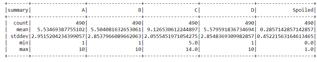
Inference: What if we want to access the statistical information about the dataset? For that, PySpark have the describe() function that is used against the chosen dataset. One can see the output where it returned the count, mean, standard deviation, minimum and maximum values of each feature, and the independent column.
Vector Assembler and Vectors in PySpark
When working with the MLIB library, we need to ensure that all the features are stacked together in one separate column, keeping the target column in another. So to attain this, PySpark comes with a VectorAssembler library that will sort things up for us without handling much manually.
from pyspark.ml.linalg import Vectors
from pyspark.ml.feature import VectorAssembler
In the above cell, we imported Vectors and VectorAssembler modules from the ml. lin and ml. feature library simultaneously. Moving forward, we will see the implementation of the same.
assembler_data = VectorAssembler(inputCols=['A', 'B', 'C', 'D'],outputCol="features")
output = assembler_data.transform(data_food)
output.show()
Output:
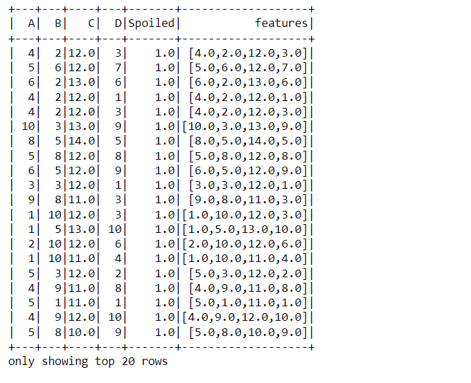
Code breakdown:
- Firstly, before using the VectorAssembler, we first need to create the object for the same, i.e., initializing it and passing the input columns (features) and output columns (the one which will be piled up)
- After initializing the object, we transform it; note that the whole dataset is passed in the parameter.
- At last, to show the transformed data show function is used, and in the output, the last column turned out to be the features column (all in one).
Model building using PySpark
Here comes the model building phase, where specifically, we will use the Tree method to achieve the motto of this article. Note that this model-building phase will not be the same as the traditional way because we don’t need the train test split instead, we just want to grab which feature has more importance.
from pyspark.ml.classification import RandomForestClassifier,DecisionTreeClassifier

rfc = DecisionTreeClassifier(labelCol='Spoiled',featuresCol='features')
Inference: Before using the tree classifiers, we need to import the random forest classifier and Decision Tree classifier from the classification module.
Then, initializing the Decision Tree object and passing in the label column (target) and features columns (feature).
final_data = output.select('features','Spoiled')
final_data.show()
Output:
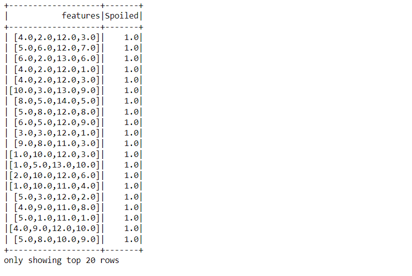
The above process of accessing only the features and target column was performed so that we can get the final data that needs to be passed in the training phase. In the output also, one can confirm the same.
rfc_model = rfc.fit(final_data)
Output:
Inference: Finally, there is the training phase, and for that fit, the method is used. Also, note that here we are passing the final data we grabbed above.
rfc_model.featureImportances
Output:
SparseVector(4, {1: 0.0019, 2: 0.9832, 3: 0.0149})
Inference: Have a close look at the output where 3 indexes are there and 2nd index has the highest value (0.9832) i.e.
Chemical C is the most important feature that stimulates Chemical C and is the main cause of the early spoilage of dog food.
Conclusion
We are in the endgame now, The last part of the article will let you summarize everything we did so far to achieve the results for which the dog food company hypothetically hired us to predict the chemical which is causing the early spoiling of the dog food.
- As usual for any Spark project here, we also set up the Spark Session and read the dataset – mandatory steps.
- Then we moved forward to the feature analysis phase and feature engineering to make the dataset ready to feed the machine learning algorithm.
- At last, we built the model (tree method), and after the same training, we grabbed the feature importance and concluded that Chemical C was mainly responsible for early spoiling.
The media shown in this article is not owned by Analytics Vidhya and is used at the Author’s discretion.


