Random Forest® vs Neural Networks for Predicting Customer Churn

Let us see how random forest competes with neural networks for solving a real world business problem.

By Abhinav Sagar, VIT Vellore on December 26, 2019 in Churn, Customer Analytics, Neural Networks, random forests algorithm

comments

Customer churn prediction is an essential requirement for a successful business. Most companies with a subscription based business regularly monitors churn rate of their customer base. Statistically 59% of customers don’t return after a bad customer service experience. In addition, cost of acquiring new customers is quite high. This makes predictive models of customer churn appealing as they enable companies to maintain their existing customers at a higher rate. Although defining and predicting customer churn might appear straightforward initially, it involves several practical challenges.

The Challenge

To make a predictive model to anticipate which customers are most likely to churn. This would help the marketing team take appropriate decisions to retain them.

Environment and tools

scikit-learn
keras
numpy
pandas
matplotlib

Data

The dataset can be downloaded from the kaggle website which can be found here.

Description of variables in the dataset:

customerID: Customer ID
gender: Whether the customer is a male or a female
SeniorCitizen: Whether the customer is a senior citizen or not (1, 0)
Partner: Whether the customer has a partner or not (Yes, No)
Dependents: Whether the customer has dependents or not (Yes, No)
tenure: Number of months the customer has stayed with the company
PhoneService: Whether the customer has a phone service or not (Yes, No)
MultipleLines: Whether the customer has multiple lines or not (Yes, No, No phone service)
InternetService: Customer’s internet service provider (DSL, Fiber optic, No)
OnlineSecurity: Whether the customer has online security or not (Yes, No, No internet service)
OnlineBackup: Whether the customer has online backup or not (Yes, No, No internet service)
DeviceProtection: Whether the customer has device protection or not (Yes, No, No internet service)
TechSupport: Whether the customer has tech support or not (Yes, No, No internet service)
StreamingTV: Whether the customer has streaming TV or not (Yes, No, No internet service)
StreamingMovies: Whether the customer has streaming movies or not (Yes, No, No internet service)
Contract: The contract term of the customer (Month-to-month, One year, Two year)
PaperlessBilling: Whether the customer has paperless billing or not (Yes, No)
PaymentMethod: The customer’s payment method (Electronic check, Mailed check, Bank transfer (automatic), Credit card (automatic))
MonthlyCharges: The amount charged to the customer monthly
TotalCharges: The total amount charged to the customer
Churn: Whether the customer churned or not (Yes or No)

Where is the code?

Without much ado, let’s get started with the code. The complete project on github can be found here.

I started with loading all the libraries and dependencies required.

import numpy as np 
import pandas as pd 
from matplotlib import pyplot as plt 
from sklearn.model_selection import train_test_split import keras 
from keras.models import Sequential 
from keras.layers import InputLayer 
from keras.layers import Dense 
from keras.layers import Dropout 
from keras.constraints import maxnorm
from sklearn.ensemble import RandomForestClassifier, RandomForestRegressor
from sklearn.metrics import classification_report, confusion_matrix, accuracy_score

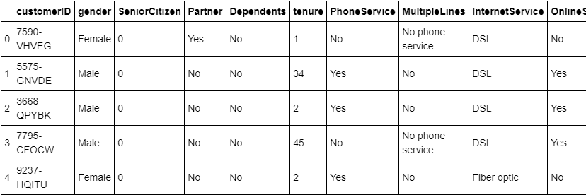
Let’s see how the dataset looks like.

read_csv is a pandas function to read csv files and do operations on it later. head() method is used to return top n (5 by default) rows of a DataFrame.

data = pd.read_csv('../input/telco-customer-churn/WA_Fn-UseC_-Telco-Customer-Churn.csv')
data.head()

Data Preprocessing

I converted the categorical variables into numerical variables (e.g. Yes/No to 1/0). I ensured that all the values are in numeric format. Also I filled null values with zero.

data.SeniorCitizen.replace([0, 1], ["No", "Yes"], inplace= True)
data.TotalCharges.replace([" "], ["0"], inplace= True)
data.TotalCharges = data.TotalCharges.astype(float)
data.drop("customerID", axis= 1, inplace= True) 
data.Churn.replace(["Yes", "No"], [1, 0], inplace= True)

pd.get_dummies creates a new dataframe which consists of zeros and ones. The dataframe will have a one depending on the truth of the categorical variables in this case.

data = pd.get_dummies(data)

Next I split the dataset into X and Y.

X contains all the features that are used for making the predictions.
Y contains the outcomes that is whether or not the customer churned

X = data.drop("Churn", axis= 1)
y = data.Churn

Next I used train_test_split to split the data into training and testing sets with 20% of the data given to the test set. The training set is used to train the model, while the test set is only used to evaluate the model’s performance.

X_train, X_test, y_train, y_test = train_test_split(X, y, test_size= 0.2, random_state= 42)

Random Forest

I used random forest classifier with 100 trees and maximum depth of trees as 20.

rf.fit builds a forest of trees from the training set (X, Y). rf.score returns the mean accuracy on the given test data and labels.

rf = RandomForestClassifier(n_estimators=100, max_depth=20,
                              random_state=42)
rf.fit(X_train, y_train) 
score = rf.score(X_train, y_train)
score2 = rf.score(X_test, y_test)
print("Training set accuracy: ", '%.3f'%(score))
print("Test set accuracy: ", '%.3f'%(score2))

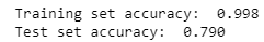
The accuracy achieved on the training set is 99.8%, while on the test set it is 79%.

rf.predict is used to predict class for X.

rf_predictions = rf.predict(X_test)
rf_probs = rf.predict_proba(X_test)

Let’s evaluate the performance of the model using some other popular classification metrics.

Confusion Matrix

Confusion Matrix is a very important metric when analyzing misclassification. Each row of the matrix represents the instances in a predicted class while each column represents the instances in an actual class. The diagonals represent the classes that have been correctly classified. This helps as we not only know which classes are being misclassified but also what they are being misclassified as.

Precision, Recall and F1-Score

For a better look at misclassification, we often use the following metric to get a better idea of true positives (TP), true negatives (TN), false positive (FP) and false negative (FN).

Precision is the ratio of correctly predicted positive observations to the total predicted positive observations.

Recall is the ratio of correctly predicted positive observations to all the observations in actual class.

F1-Score is the weighted average of Precision and Recall.

y_pred = rf.predict(X_test)
print(confusion_matrix(y_test,y_pred))
print(classification_report(y_test,y_pred))
print(accuracy_score(y_test, y_pred))

The performance metrics are quite good for predicting customers who dosen’t churn with precision, recall and F1 score values of 0.83, 0.91,0.86. But the problem is that model is not able to accurately predict the customers who will churn with the corresponding values of 0.64, 0.47, 0.54.

I continued with identifying which features are important for the problem in hand. This can help in early detection and maybe even improve the business strategy.

fi = pd.DataFrame({'feature': list(X_train.columns),
                   'importance': rf.feature_importances_}).\
                    sort_values('importance', ascending = False)
fi.head()

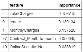
It can be seen that the most important feature for our prediction problem is TotalCharges followed by tenure and MonthlyCharges.

Neural Networks

Now let’s code a neural network for the same problem. I used a very simple neural network. Please note that the data is in tabular format, hence we don’t need to use complicated architectures which would lead to overfitting.

I used two dense layers with 64 neurons and 8 neurons with relu as the activation function. input_dim argument denotes the number of features in the dataset or in other words the number of columns present in the dataset. In between, I used 20% dropouts to reduce overfitting. The dropout layer ensures that we remove a set percentage of the data each time we iterate through the neural network. kernel_constraint is used for scaling of the weights present in the neural network. The last layer is also a dense layer with 1 neuron and sigmoid as the activation function.

model = Sequential()
model.add(Dense(64, input_dim=46, activation='relu', kernel_constraint=maxnorm(3)))
model.add(Dropout(rate=0.2))
model.add(Dense(8, activation='relu', kernel_constraint=maxnorm(3)))
model.add(Dropout(rate=0.2))
model.add(Dense(1, activation='sigmoid'))

Next I compiled the model using binary_crossentropy as the loss function, adam as the optimizer and accuracy metric to track during training.

model.compile(loss = "binary_crossentropy", optimizer = 'adam', metrics=['accuracy'])

I trained the model for 50 epochs with a batch size value of 8. One epoch is when an entire dataset is passed forward and backward through the neural network only once. Batch size is the total number of training examples present in a single batch.

history = model.fit(X_train, y_train, validation_data=(X_test, y_test), epochs=50, batch_size=8)

Now let’s see how accuracy varies as a function of epochs.

plt.plot(history.history['accuracy']) 
plt.plot(history.history['val_accuracy']) 
plt.title('model accuracy') 
plt.ylabel('accuracy')
plt.xlabel('epoch') 
plt.legend(['train', 'test'], loc='upper left') 
plt.show()

Accuracy vs epochs

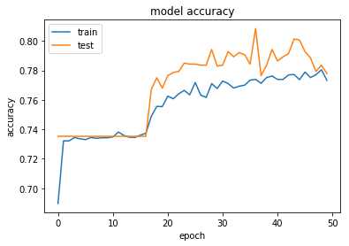
The test accuracy of the neural network after 50 epochs is 78% which is comparable to the 79% accuracy of the random forest.

Conclusions

In this article, I demonstrated how a business can predict and retain their customers. I compared random forest and neural networks for the same. The accuracy of both the algorithms are comparable, hence it is hard to tell which is better. Random forest has proven to be a great algorithm if the dataset is in tabular format. Random Forests requires less preprocessing and the training process is also much simpler. Also hyper-parameter tuning is easier with random forest when compared to neural networks. This gives random forest the edge above neural networks.

References/Further Readings

Hands-on: Predict Customer Churn
Long story short — in this article we want to get our hands dirty: building a predictivmodel that identifies customers…

Predict Customer Churn - Logistic Regression, Decision Tree and Random Forest
Customer churn occurs when customers or subscribers stop doing business with a company or service, also known as…

Customer churn prediction in telecommunication industry using data certainty
JavaScript is disabled on your browser. Please enable JavaScript to use all the features on this page. Customer Churn…

Before You Go

The corresponding source code can be found here.

abhinavsagar/Machine-Learning-Projects
You can't perform that action at this time. You signed in with another tab or window. You signed out in another tab or…

Contacts

If you want to keep updated with my latest articles and projects follow me on Medium. These are some of my contacts details:

Happy reading, happy learning and happy coding!

Bio: Abhinav Sagar is a senior year undergrad at VIT Vellore. He is interested in data science, machine learning and their applications to real-world problems.

Original. Reposted with permission.

Related:

RANDOM FORESTS and RANDOMFORESTS are registered marks of Minitab, LLC.