Data Science Interview Part 3: ROC-AUC
This article was published as a part of the Data Science Blogathon.
Introduction
<strong>Python Code:</strong> <div class="coding-window"><iframe width="100%" height="1400px" frameborder="no" scrolling="no" sandbox="allow-forms allow-pointer-lock allow-popups allow-same-origin allow-scripts allow-modals" allowfullscreen="allowfullscreen" data-src="https://repl.it/@Santhosh-Reddy1/AUC-ROC?lite= true"><span data-mce-type="bookmark" style="display: inline-block; width: 0px; overflow: hidden; line-height: 0;" class="mce_SELRES_start"></ span></iframe></div>
ROC – AUC CURVE
y = loan_df['Loan_Status']

X = loan_df.drop(['Loan_ID', 'Loan_Status'], axis = 1)

lbe = LabelEncoder()

y_labeled = lbe.fit_transform(y)

from sklearn.model_selection import train_test_split as tst

X_train, X_valid, y_train, y_valid = tst(X, y_labeled, test_size = 0.25, stratify = y_labeled)

model = LogisticRegression()

model.fit(X_train, y_train)
y_preds = model.predict_proba(X_valid)
from sklearn.metrics import roc_curve

# retrieving just the probabilities for the positive class

pos_probs = y_preds[:, 1]

# plotting no skill roc curve

plt.plot([0, 1], [0, 1], linestyle='--', label='No Skill')

# calculating roc curve for model

fpr, tpr, _ = roc_curve(y_valid, pos_probs)

# plotting model roc curve

plt.plot(fpr, tpr, marker='.', label='Logistic')

# assigning axis labels

plt.xlabel('False Positive Rate')

plt.ylabel('True Positive Rate')

# show the legend

plt.legend()

# show the plot

plt.show()
from sklearn.metrics import roc_auc_score

# calculate roc auc

roc_auc = roc_auc_score(y_valid, pos_probs)

print('Logistic ROC AUC %.3f' % roc_auc)
What is Hyperparameter Tuning? Can you explain any tuning method?
We use the Hyperparameter tuning technique to get the best hyperparameters for the model. The hyperparameters are the parameters that are available in the Machine Learning algorithm.
There are various techniques to perform Hyperparameter tuning, and we will discuss the implementation of each method with the running example.
Let’s first install Scikit Optimize for BayesianSearchCV and Xgboost for the Xgboost classifier.
!pip install scikit_optimize xgboost
from xgboost import XGBClassifier
from sklearn.model_selection import GridSearchCV, RandomizedSearchCV, StratifiedShuffleSplit
from scipy.stats import randint, uniform
from skopt import BayesSearchCV
from skopt.space import Real, Categorical, Integer
GridSearchCV
We, as data scientists, often use this method to get the best hyperparameters. This method performs the training with all possible hyperparameter permutations for a model. Then we evaluate the performance of each permutation and select the best model.
Since GridSearchCV uses all combinations of the hyperparameters hence, it is highly computationally expensive.
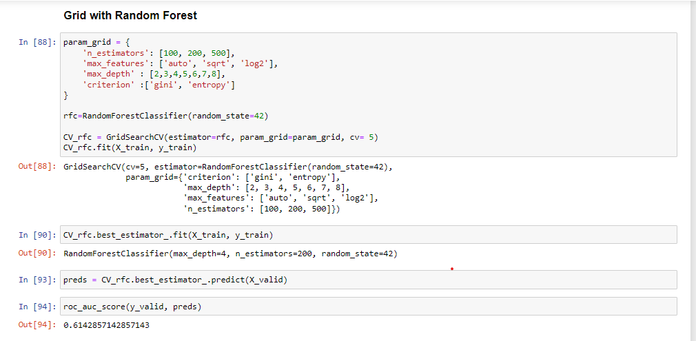
In this project, we will build a classification model using GridSearchCV with Xgboost and Random Forest.
%%time
param = {
    'learning_rate': [.1]
    , 'subsample': [.2, .3 ,.4, .5]
    , 'n_estimators': [25, 50]
    , 'min_child_weight': [25]
    , 'reg_alpha': [.3, .4, .5]
    , 'reg_lambda': [.1, .2, .3, .4, .5]
    , 'colsample_bytree': [.66]
    , 'max_depth': [5]
}
#iter - 4x2x3x5 = 120
model = XGBClassifier(random_state=42, n_jobs=-1) #input hyperparameters without tuning
gridsearch = GridSearchCV(model, param_grid=param, cv=3, n_jobs=-1, scoring='accuracy', return_train_score=True)
gridsearch.fit(X, y_labeled)
print('best score of Grid Search over 120 iterations:', gridsearch.best_score_)
The code shows the implementation of GridSearchCV with the Xgboost classifier. The model-building process starts with initializing parameters, and then GridSearchCV finds the best suitable hyperparameters for Xgboost by permutations and combinations of the hyperparameters.
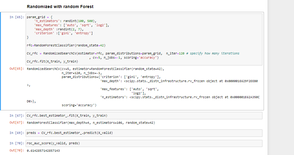
RandomizedSearchCV
Randomized SearchCV uses a list or statistical distribution of hyperparameters instead of a set of discrete values and picks the hyperparameter values randomly from the distribution.
Note:
GridSearchCV is more applicable for small datasets, while for the large dataset, we should go for RandomizedSearchCV to reduce the computation complexity.
%%time
param = {
    'learning_rate': uniform(.05, .1) #actual value: (loc, loc + scale)
    , 'subsample': uniform(.2, .3)
    , 'n_estimators': randint(20, 70)
    , 'min_child_weight': randint(20, 40)
    , 'reg_alpha': uniform(0, .7)
    , 'reg_lambda': uniform(0, .7)
    , 'colsample_bytree': uniform(.1, .7)
    , 'max_depth': randint(2, 6)
}
randomsearch = RandomizedSearchCV(model, param_distributions=param, n_iter=120 # specify how many iterations
                                  , cv=3, n_jobs=-1, scoring='accuracy', return_train_score=True)
randomsearch.fit(X, y_labeled)
print('best score of Randomized Search over 120 iterations:', randomsearch.best_score_)
The above code is for the Randomized Search CV with the Xgboost running for 120 iterations. The first step is to initialize the parameters in statistical distributions and then train the model with Randomly picked hyperparameters.
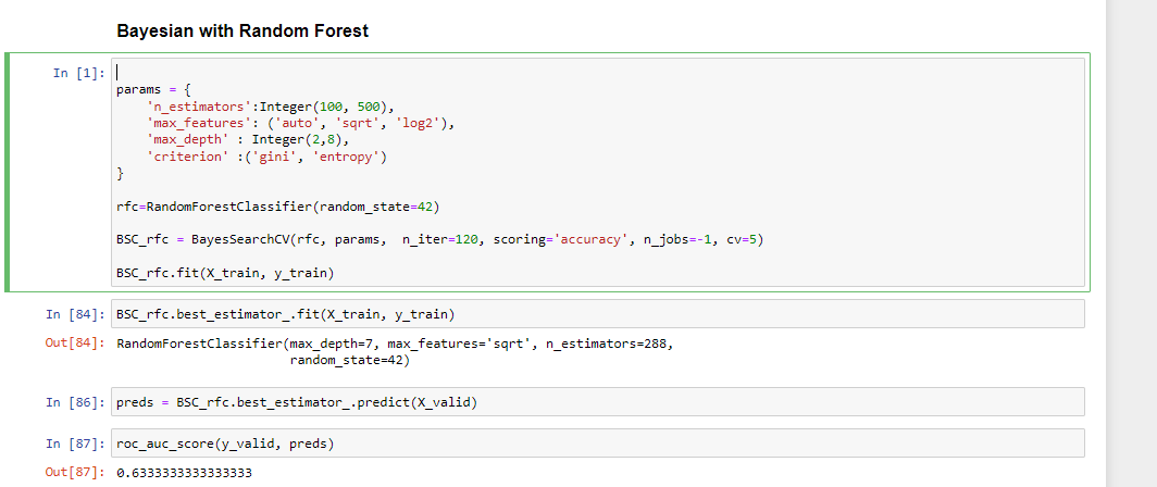
BayesianSearchCV
BayasianSearchCV technique uses Bayesian optimization for exploring the most appropriate hyperparameters for the ML model. It minimizes the acquisition function using Gaussian Process Regression on the acquisition function. BayesianSearchcv keeps track of past evaluation results and uses them to form a probabilistic model mapping hyperparameters to a probability of a score on the objective function.
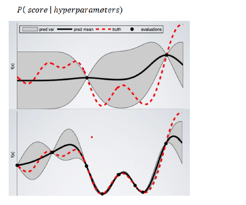
Moreover, we can feed a wide range of parameter values into Bayesian optimization. Because it automatically explores the most appropriate regions and discards the unpromising ones.
The objective function here is to get the best predictions using the specified model hyperparameters.
%%time
param = {
    'learning_rate': Real(.05, .1+.05) #lower bound and upper bound
    , 'subsample': Real(.2, .5)
    , 'n_estimators': Integer(20, 70)
    , 'min_child_weight': Integer(20, 40)
    , 'reg_alpha': Real(0, 0+.7)
    , 'reg_lambda': Real(0, 0+.7)
    , 'colsample_bytree': Real(.1, .1+.7)
    , 'max_depth': Integer(2, 6)
}
bayessearch = BayesSearchCV(model, param, n_iter=60, # specify how many iterations
                                    scoring='accuracy', n_jobs=-1, cv=3)
bayessearch.fit(X, y_labeled)
print('best score of Bayes Search over 60 iterations:', bayessearch.best_score_)
The code is for training the BayesianSearchCV with Xgboost and its hyperparameters. The BayesianSearchCV trains the Xgboost over 60 iterations with the predefined hyperparameters range. The BayesianSearchCV will determine the best hyperparameters using Bayesian Optimization while minimizing the acquisition rate.
Results:
| Model Name | ROC AUC Score |
| GridSearchCV with XGBoost Classifier | 0.5 |
| RandomizedSearchCV with XGBoost Classifier | 0.5 |
| BayesianSearchCV with XGBoost Classifier | 0.5 |
You will find the notebook here for detailed implementation.
What is ZCA Whitening?
ZCA stands for Zero Component Analysis which converts the co-variance matrix into an Identity matrix. This process removes the statistical structure from the first and second-order structures.
We can use ZCA to drive the features linearly independent of each other and transform the data toward a zero mean. We can apply ZCA whitening to the small colored images before training an image classification model. This technique gets used in Image Augmentation to create more complex picture patterns so that the model can also classify blurred and whitened images.
We will try implementing the ZCA Whitening to understand using the Mnist dataset.
1 2 3 4 5 6 7 8 9 10 11 12 13 14 15 16 17 18 19 20 21 22 23 25 26 27 28 24 |
# ZCA Whitening from tensorflow.keras.datasets import mnist
from tensorflow.keras.preprocessing.image import ImageDataGenerator
import matplotlib.pyplot as plt
# load data
(X_train, y_train), (X_test, y_test) = mnist.load_data()
# reshape to be [samples][width][height][channels]
X_train = X_train.reshape((X_train.shape[0], 28, 28, 1))
X_test = X_test.reshape((X_test.shape[0], 28, 28, 1))
# convert from int to float
X_train = X_train.astype('float32')
X_test = X_test.astype('float32')
# define data preparation
datagen = ImageDataGenerator(featurewise_center=True, featurewise_std_normalization=True, zca_whitening=True)
# fit parameters from data
X_mean = X_train.mean(axis=0)
datagen.fit(X_train - X_mean)
# configure batch size and retrieve one batch of images
for X_batch, y_batch in datagen.flow(X_train - X_mean, y_train, batch_size=9, shuffle=False):
print(X_batch.min(), X_batch.mean(), X_batch.max())
# create a grid of 3x3 images
fig, ax = plt.subplots(3, 3, sharex=True, sharey=True, figsize=(4,4))
for i in range(3):
for j in range(3):
ax[i][j].imshow(X_batch[i*3+j].reshape(28,28), cmap=plt.get_cmap("gray"))
# show the plot
plt.show()
break
|
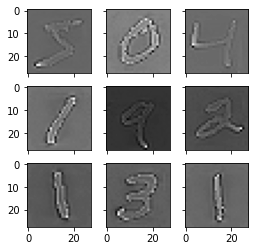
The outline of each image has been highlighted after applying ZCA Whitening using TensorFlow and ImageDatagenerator, as shown in the image above.
Conclusion
We have discussed some more interview questions around ZCA Whitening, Hyperparameter Tuning, and ROC-AUC. We have seen that among all the hyperparameter tuning techniques, BayesSearchCV performed well with a ROC AUC Score of .68.
However, it can not be considered the final result.
Let us summarise the blog with some key takeaways:
- ROC AUC metric is effective with imbalanced classification problems.
- ROC curve plots the correlation of True Positive Rate with False Negative Rate.
- AUC is the area under the ROC curve and gets used when ROC curve results are not interpretable.
- GridSearchCV uses permutations of all the hyperparameters, making it computationally expensive.
- RandomizedSearchCV selects random hyperparameter combinations from the statistical distribution.
- BayesSearchCV chooses hyperparameters with Bayesian optimization.
- ZCA Whitening makes the features linearly independent and reduces the data mean to zero.
- ZCA whitening is applicable for tiny colored images to remove the co-relation from the first and second-order statistical structure.
That takes us to the end of this blog. I hope you find this article valuable and comprehensive. If you can, please do share this blog with your friends. For any doubt, query, feedback, or topic suggestion, reach me on my Linkedin.
The media shown in this article is not owned by Analytics Vidhya and is used at the Author’s discretion.


