Introduction

Diabetes is usually classified into 2- type 1 and type 2. Diabetes mellitus, which is Type 2 diabetes, is a chronic condition posing significant challenges to global healthcare systems. The increasing prevalence of this disease demands innovative approaches for early detection and effective management. Recent advancements in artificial intelligence and machine learning techniques offer promising solutions for predicting diabetes. Utilizing extensive datasets, including essential health indicators such as blood pressure, body mass index (BMI), and glucose levels, machine learning models can identify patterns and risk factors associated with diabetes.

In this context, various machine learning algorithms, including decision trees, random forests, support vector machines (SVM), and neural networks, have been employed to develop robust classifiers for diabetes prediction. Notably, algorithms such as logistic regression, Naive Bayes, and k-nearest neighbors (KNN) have shown significant potential in the prediction of type 1 or type 2 diabetes in prediabetic patients.

The deployment of these models in real-world healthcare settings can facilitate early diagnosis and intervention, potentially reducing the burden of diabetes-related complications. This article delves into the methodologies, data analysis, and evaluation metrics of different machine-learning approaches for diabetes prediction, highlighting their implications in clinical practice and public health. Through systematic review and performance analysis, we aim to provide a comprehensive overview of the current landscape for early detection of diabetes and future directions in using machine learning for diabetes prediction models.

Learning Outcome

1. Learn diabetes prediction using machine learning, covering data prep, model selection, and result interpretation.
2. Understand preprocessing techniques and model evaluation metrics for accurate predictions.
3. Gain insight into popular algorithms like Random Forest and support vector machines (SVM) for diabetes prediction.
4. Interpret model results for informed decision-making for early prediction of diabetes disease prediction in healthcare applications.

This article was published as a part of the Data Science Blogathon.

What is EDA?

Exploratory Data Analysis (EDA) is a crucial step in the data analysis process, aimed at summarizing the main characteristics of a dataset, often with visual methods. Here are the critical aspects of EDA:

1. Data Cleaning involves identifying and handling missing values, duplicates, and outliers. This step ensures that the data is accurate and ready for analysis.
2. Descriptive Statistics involves calculating measures such as mean, median, mode, standard deviation, and range to understand the distribution and central tendencies of the data.
3. Data Visualization involves creating plots like histograms, scatter plots, box plots, and bar charts to inspect the data visually. It helps identify patterns, correlations, and anomalies.
4. Transformation and Aggregation: Applying transformations such as log, square root, or normalization to stabilize variance and aggregate data to understand it at different levels.
5. Feature Engineering: Creating new features from existing data to improve the performance of machine learning models.
6. Pattern Detection involves looking for trends, correlations, and interactions between variables that can provide insights or suggest hypotheses.

EDA is iterative and involves going back and forth between different steps to refine the understanding of the data. The goal is to make sense of the data, detect essential features, and generate questions or hypotheses for further analysis. It is an integral part of data science and helps make informed decisions for subsequent data modeling and analysis steps.

What is Machine Learning?

Machine learning (ML) is a subset of artificial intelligence (AI) that focuses on building systems to learn from and make data-based decisions. Instead of being explicitly programmed to perform a task, these systems use algorithms to identify patterns and make predictions or decisions. Here are the key components and types of machine learning:

Critical Components of Machine Learning:

1. Data: The foundation of machine learning, including training data (used to train the model) and test data (used to evaluate the model’s performance).
2. Algorithms are rules or procedures used to perform calculations, process data, and make decisions. Common algorithms include decision trees, support vector machines, and neural networks.
3. Models: The training process output represents patterns learned from the data.
4. Training: The process of feeding data to an algorithm to learn the relationships within the data.
5. Evaluation: Assessing the model’s performance using accuracy, precision, recall, and F1 score metrics.

Types of Machine Learning:

Supervised Learning: The model is trained on labeled data, where the input data and the corresponding output are provided. For example, regression (predicting continuous values) and classification (categorizing data into discrete classes) are used. Its applications are Spam detection, image classification, and medical diagnosis.

Unsupervised Learning: The model is trained on unlabeled data and must find patterns and relationships within the data. For example, Clustering (grouping similar data points) and association (finding rules that describe large portions of data). Its applications are Customer segmentation, market basket analysis, and anomaly detection.

Semi-supervised Learning: It combines a small amount of labeled data with many unlabeled data during training. Its applications are situations where acquiring labeled data is expensive or time-consuming, such as medical image analysis.

Reinforcement Learning: The model learns by interacting with an environment and receiving rewards or penalties based on its actions. For example, algorithms for playing games, robotic control, and self-driving cars. Its applications are Game playing (like AlphaGo), robotics, and recommendation systems.

Also Read: Supervised Learning And Unsupervised Machine Learning

Why is Machine Learning Better for Diabetes Prediction than Other Models?

Machine learning offers several advantages over traditional statistical models and other methods for diabetes prediction, making it particularly well-suited for this application. Here are key reasons why machine learning is often better for diabetes prediction:

1. Handling Complex and Non-linear Relationships

Machine learning algorithms, such as decision trees, random forests, and neural networks, excel at capturing complex, non-linear relationships between features that traditional linear models might miss.

Example: The relationship between blood glucose levels, age, BMI, and diabetes risk is often non-linear and may involve complex interactions that machine learning models can better capture.

2. Feature Engineering and Selection

Machine learning models can automatically perform feature selection and engineering, identifying the most relevant features for predicting diabetes.

Example: Algorithms like LASSO (Least Absolute Shrinkage and Selection Operator) or random forests can rank features by importance, potentially uncovering hidden predictors of diabetes.

3. Handling Large and Diverse Datasets

Machine learning models can handle large datasets with many features and observations, improving the predictions’ robustness and accuracy.

Example: With access to extensive patient records, including medical history, lifestyle factors, and genetic information, machine learning models can provide more accurate predictions than models limited to smaller datasets.

4. Adaptability to New Data

Machine learning models, particularly in dynamic environments, can be updated and retrained with new data to improve their accuracy and adapt to population or disease characteristics changes.

Example: As new research reveals more about the genetic markers associated with diabetes, machine learning models can incorporate this information to enhance prediction accuracy.

5. Integration of Various Data Types

Machine learning models can integrate and analyze diverse data types, including structured data (e.g., lab results) and unstructured data (e.g., doctor’s notes, medical imaging).

Example: Combining lab results, lifestyle information, and genomic data in a single model can lead to more comprehensive and accurate diabetes predictions.

6. Improved Predictive Performance

Machine learning models generally outperform traditional models in predictive accuracy due to their ability to learn from large datasets and capture complex patterns.

Example: Studies have shown that machine learning models, like gradient boosting machines or deep neural networks, often provide higher accuracy in diabetes prediction compared to logistic regression.

7. Early Detection and Prevention

Machine learning models can identify high-risk individuals earlier than traditional methods, enabling timely interventions and potentially preventing the onset of diabetes.

Example: Early identification through predictive modeling can lead to lifestyle modifications or medical treatments that delay or prevent diabetes.

What is Diabetes Prediction Using Machine Learning?

Diabetes prediction using machine learning means using computer programs to guess if someone might get diabetes. These programs look at things like health history and lifestyle to make their guess. They learn from many examples of people with and without diabetes to make better guesses. For instance, they might look at how much sugar someone eats or if they exercise regularly. By doing this, they can give early warnings to people at risk of getting diabetes so they can take better care of themselves.

The Dataset

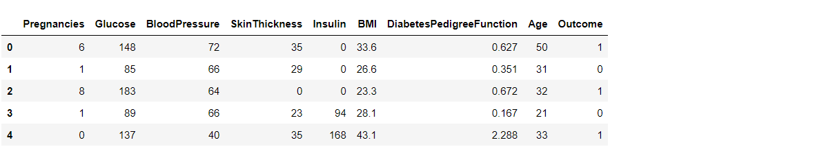
The Pima Indians Diabetes Dataset is a publicly available test dataset widely used for diabetes research and predictive modeling. It contains 768 observations of females of Pima Indian heritage aged 21 years or older. The dataset includes eight medical predictor variables and one target variable. The predictor variables are:

• Pregnancies: Number of times pregnant
• Glucose: Plasma glucose concentration over 2 hours in an oral glucose tolerance test
• Blood Pressure: Diastolic blood pressure (mm Hg)
• Skin Thickness: Triceps skinfold thickness (mm)
• Insulin: 2-hour serum insulin (mu U/ml)
• BMI: Body mass index (weight in kg/(height in m)^2)
• Diabetes Pedigree Function: A function that scores the likelihood of diabetes based on family history
• Age: Age in years

The target variable is ‘Outcome’’ which indicates whether the patient had diabetes (1) or not (0). This training dataset is particularly useful for testing machine learning algorithms for binary classification tasks.

Importing Libraries

import numpy as np
import pandas as pd
import matplotlib.pyplot as plt
import seaborn as sns

sns.set()

from mlxtend.plotting import plot_decision_regions
import missingno as msno
from pandas.plotting import scatter_matrix
from sklearn.preprocessing import StandardScaler
from sklearn.model_selection import train_test_split
from sklearn.neighbors import KNeighborsClassifier

from sklearn.metrics import confusion_matrix
from sklearn import metrics
from sklearn.metrics import classification_report
import warnings
warnings.filterwarnings('ignore')
%matplotlib inline

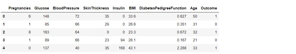
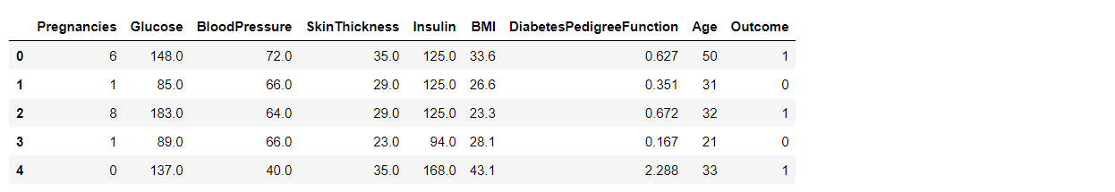
We start by reading the training dataset, which is in CSV format:

diabetes_df = pd.read_csv('diabetes.csv') diabetes_df.head()

Output:

Exploratory Data Analysis (EDA)

Exploring Dataset Columns

First, let’s see the columns available in our dataset:

diabetes_df.columns

Output:

Index(['Pregnancies', 'Glucose', 'BloodPressure', 'SkinThickness', 'Insulin', 'BMI', 'DiabetesPedigreeFunction', 'Age', 'Outcome'], dtype='object')

Dataset Information

To get more information about the dataset:

diabetes_df.info()

Output:

RangeIndex: 768 entries, 0 to 767
Data columns (total 9 columns):
 #   Column                   Non-Null Count  Dtype  
---  ------                   --------------  -----  
 0   Pregnancies              768 non-null    int64  
 1   Glucose                  768 non-null    int64  
 2   BloodPressure            768 non-null    int64  
 3   SkinThickness            768 non-null    int64  
 4   Insulin                  768 non-null    int64  
 5   BMI                      768 non-null    float64
 6   DiabetesPedigreeFunction 768 non-null    float64
 7   Age                      768 non-null    int64  
 8   Outcome                  768 non-null    int64  
dtypes: float64(2), int64(7)
memory usage: 54.1 KB

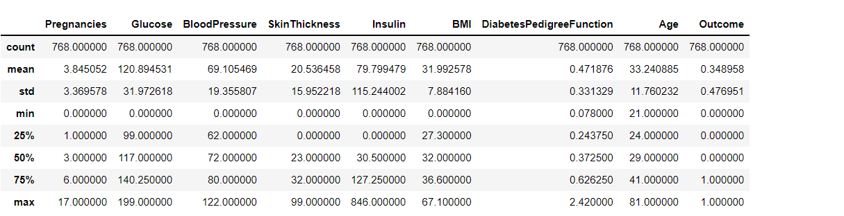
Dataset Description

To understand the statistics of the dataset:

diabetes_df.describe()

Output:

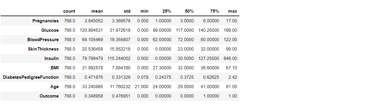
To know more about the dataset with transpose – here, T is for the transpose

diabetes_df.describe().T

Output:

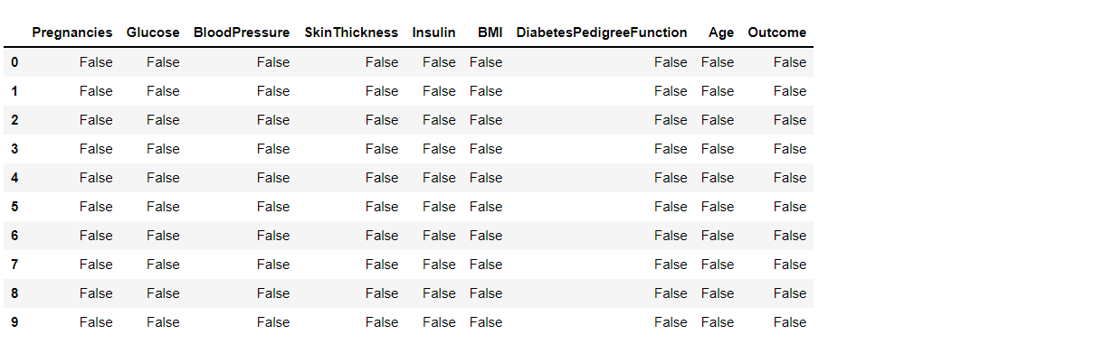
Checking for Null Values

Let’s check if our dataset has any null values:

diabetes_df.isnull().head(10)

Output:

To get the total number of null values in the dataset:

diabetes_df.isnull().sum()

Output:

Pregnancies                 0
Glucose                     0
BloodPressure               0
SkinThickness               0
Insulin                     0
BMI                         0
DiabetesPedigreeFunction    0
Age                         0
Outcome                     0
dtype: int64

We observe no missing values from the above code, which is misleading. In this dataset, missing values are encoded as 0. Therefore, we must replace the 0 values with NaN and then blame them properly.

Handling Missing Values

Replace 0 values with NaN:

diabetes_df_copy = diabetes_df.copy(deep=True)
diabetes_df_copy[['Glucose', 'BloodPressure', 'SkinThickness', 'Insulin', 'BMI']] = diabetes_df_copy[['Glucose', 'BloodPressure', 'SkinThickness', 'Insulin', 'BMI']].replace(0, np.NaN)

# Showing the count of NaNs
print(diabetes_df_copy.isnull().sum())

Output:

Pregnancies                  0
Glucose                      5
BloodPressure               35
SkinThickness              227
Insulin                    374
BMI                         11
DiabetesPedigreeFunction     0
Age                          0
Outcome                      0
dtype: int64

We will replace the zeros with NaN values to maintain the dataset’s authenticity and then attribute these missing values to the respective columns’ mean or median.

Data Visualization

Data Distribution Before Imputing Missing Values

First, let’s visualize the distribution of each feature in the dataset before removing null values:

p = diabetes_df.hist(figsize=(20, 20))

Output:

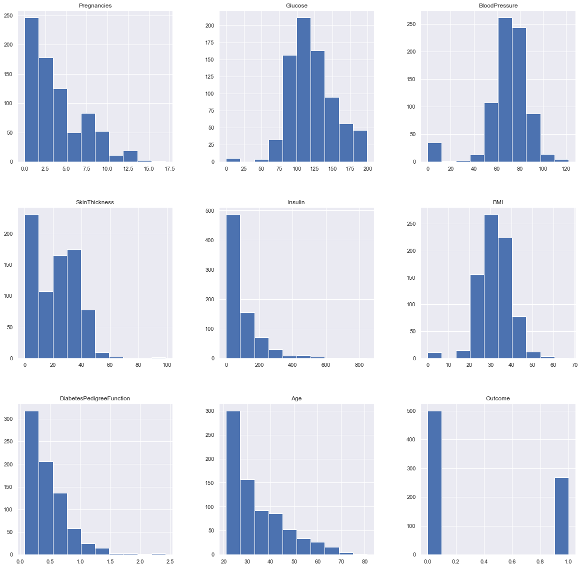
So here, we have seen the distribution of each feature, whether dependent or independent. One thing that could always strike us is why we need to know the distribution of data.? So; the answer is simple: it is the best way to start the dataset analysis as it shows the occurrence of every value in the graphical structure, letting us know the range of the data.

Imputing Missing Values

Now, we will attribute the missing values. We’ll use the mean value for ‘Glucose’ and ‘BloodPressure’’ and the median value for ‘SkinThickness’’ ‘Insulin’’ and ‘BMI’:

diabetes_df_copy['Glucose'].fillna(diabetes_df_copy['Glucose'].mean(), inplace=True)
diabetes_df_copy['BloodPressure'].fillna(diabetes_df_copy['BloodPressure'].mean(), inplace=True)
diabetes_df_copy['SkinThickness'].fillna(diabetes_df_copy['SkinThickness'].median(), inplace=True)
diabetes_df_copy['Insulin'].fillna(diabetes_df_copy['Insulin'].median(), inplace=True)
diabetes_df_copy['BMI'].fillna(diabetes_df_copy['BMI'].median(), inplace=True)

Data Distribution After Imputing Missing Values

Let’s visualize the distribution of each feature again after imputing the missing values:

p = diabetes_df_copy.hist(figsize=(20, 20))

Output:

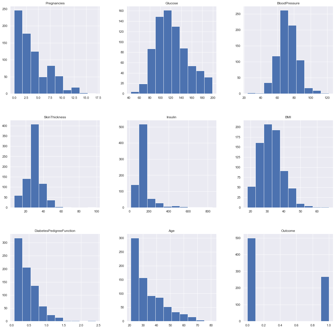
Inference: Here we are again using the hist plot to see the distribution of the dataset, but this time, we are using this visualization to see the changes that we can see after those null values are removed from the dataset, and we can see the difference for example – In age column after removal of the null values, we can see that there is a spike at the range of 50 to 100 which is quite logical as well.

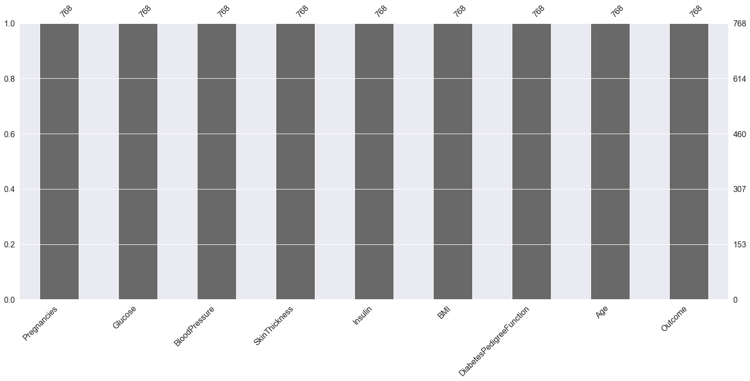
Null Count Analysis

To further verify that there are no null values left in the dataset, we can use the Missingno library:

p = msno.bar(diabetes_df)

Output:

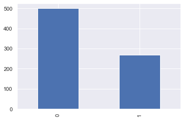
color_wheel = {1: "#0392cf", 2: "#7bc043"}
colors = diabetes_df["Outcome"].map(lambda x: color_wheel.get(x + 1))
print(diabetes_df.Outcome.value_counts())
p = diabetes_df.Outcome.value_counts().plot(kind="bar")

Output:

0    500
1    268
Name: Outcome, dtype: int64

Inference: The above visualization indicates that our training dataset is imbalanced. The number of non-diabetic patients is almost double that of diabetic patients.

Output

Distribution and Outliers of Insulin

Finally, let’s examine the distribution and outliers for the ‘Insulin’ feature using both a distplot and a boxplot:

plt.subplot(121)
sns.distplot(diabetes_df['Insulin'])
plt.subplot(122)
diabetes_df['Insulin'].plot.box(figsize=(16, 5))
plt.show()

Output:

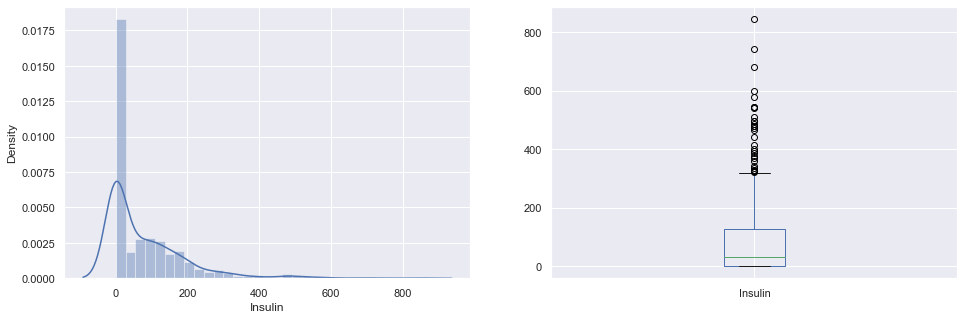
Inference: The distplot helps us understand the distribution of the ‘Insulin’ feature, while the boxplot reveals any outliers present. This combined approach provides a comprehensive view of the data, highlighting any potential issues that need to be addressed during further analysis.

Correlation between all the features

Let’s analyze the correlation between all the features in the dataset before any data cleaning. This will help us understand the relationships between different features:

plt.figure(figsize=(12, 10))
# Using seaborn to create a heatmap for the correlation matrix
p = sns.heatmap(diabetes_df.corr(), annot=True, cmap='RdYlGn')

Output:

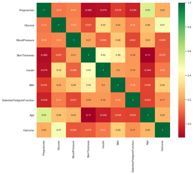
Inference: The heatmap above shows the correlation coefficients between each pair of features in the dataset. The correlation coefficient ranges from -1 to 1, where:

• 1 indicates a perfect positive correlation,
• -1 indicates a perfect negative correlation,
• 0 indicates no correlation.

By examining the heatmap, we can identify which features strongly correlate with each other and with the target variable ‘Outcome’’ This information is crucial for feature selection and engineering steps in the machine learning pipeline.

Scaling the Data

Previewing the Data Before Scaling

Before scaling the data, let’s take a quick look at the first few rows of the testing data:

diabetes_df_copy.head()

Output:

Applying Standard Scaling

Next, we will apply standard scaling to the training dataset. Standard scaling helps normalize the data, ensuring that each feature contributes equally to the machine-learning model:

from sklearn.preprocessing import StandardScaler

sc_X = StandardScaler()
X = pd.DataFrame(sc_X.fit_transform(diabetes_df_copy.drop(['Outcome'], axis=1)), 

columns=['Pregnancies', 'Glucose', 'BloodPressure', 'SkinThickness', 'Insulin', 'BMI', 'DiabetesPedigreeFunction', 'Age'])

X.head()

Output:

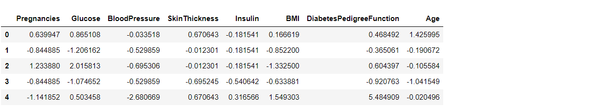
After scaling, the values of all features are now on the same scale. This helps our machine learning model perform better because no single feature will dominate due to its larger values.

Exploring the Target Column

Let’s also take a look at our target variable, ‘Outcome’:

y = diabetes_df_copy.Outcome
y.head()

Output:

0    1
1    0
2    1
3    0
4    1
Name: Outcome, dtype: int64

The ‘Outcome’ column shows whether a patient has diabetes (1) or not (0). Understanding the target variable is essential to build an accurate predictive model.

Model Building

Splitting the Dataset

First, we need to split the dataset into features (X) and target (y):

X = diabetes_df.drop('Outcome', axis=1)
y = diabetes_df['Outcome']

Now, we will split the data into training and testing sets using the train_test_split Function:

from sklearn.model_selection import train_test_split

X_train, X_test, y_train, y_test = train_test_split(X, y, test_size=0.33, random_state=7)

Random Forest

Building the model using Random Forest:

from sklearn.ensemble import RandomForestClassifier

rfc = RandomForestClassifier(n_estimators=200)
rfc.fit(X_train, y_train)

Check the accuracy of the model on the training dataset:

rfc_train = rfc.predict(X_train)
from sklearn import metrics
print("Training Accuracy =", format(metrics.accuracy_score(y_train, rfc_train)))

Output:

Training Accuracy = 1.0

The model is overfitted on the training data. Now, let’s check the accuracy of the test data:

predictions = rfc.predict(X_test)
print("Test Accuracy =", format(metrics.accuracy_score(y_test, predictions)))

Output:

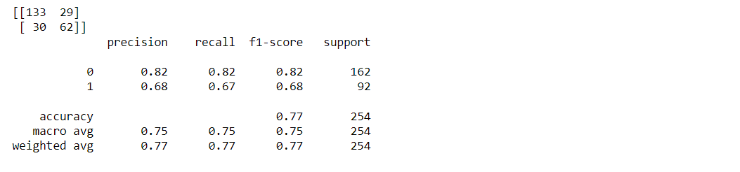
Test Accuracy = 0.7677165354330708

Get the classification report and confusion matrix:

from sklearn.metrics import classification_report, confusion_matrix

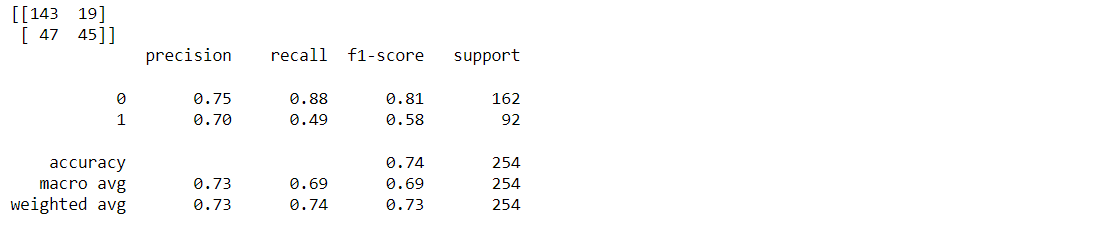
print(confusion_matrix(y_test, predictions))
print(classification_report(y_test, predictions))

Output:

Decision Tree

Building the model using a Decision Tree:

from sklearn.tree import DecisionTreeClassifier

dtree = DecisionTreeClassifier()
dtree.fit(X_train, y_train)

Make predictions on the testing data:

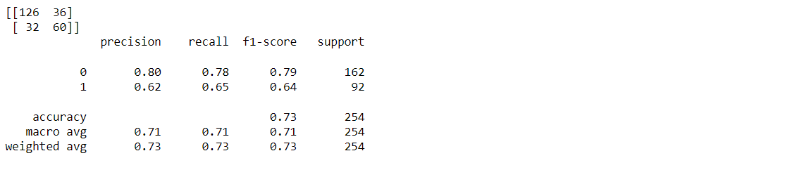
predictions = dtree.predict(X_test)
print("Test Accuracy =", format(metrics.accuracy_score(y_test, predictions)))

Output:

Test Accuracy = 0.7322834645669292

Get the classification report and confusion matrix:

from sklearn.metrics import classification_report, confusion_matrix

print(confusion_matrix(y_test, predictions))
print(classification_report(y_test, predictions))

Output:

XgBoost Classifier

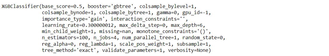
from xgboost import XGBClassifier

xgb_model = XGBClassifier(gamma=0)
xgb_model.fit(X_train, y_train)

Output:

Make predictions on the testing data:

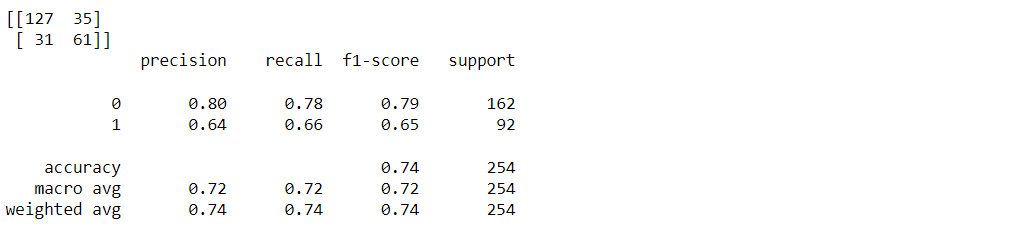
xgb_pred = xgb_model.predict(X_test)
print("Test Accuracy =", format(metrics.accuracy_score(y_test, xgb_pred)))

Output:

Test Accuracy = 0.7401574803149606

Get the classification report and confusion matrix:

from sklearn.metrics import classification_report, confusion_matrix

print(confusion_matrix(y_test, xgb_pred))
print(classification_report(y_test, xgb_pred))

Output:

Support Vector Machine (SVM)

from sklearn.svm import SVC

svc_model = SVC()
svc_model.fit(X_train, y_train)

Make predictions on the testing data:

svc_pred = svc_model.predict(X_test)
print("Test Accuracy =", format(metrics.accuracy_score(y_test, svc_pred)))

Output:

Test Accuracy = 0.7401574803149606

Get the classification report and confusion matrix:

from sklearn.metrics import classification_report, confusion_matrix

print(confusion_matrix(y_test, svc_pred))
print(classification_report(y_test, svc_pred))

Output:

Model Performance Comparison

https://drive.google.com/file/d/14k4n5AITakLFs39fZGKwGFkVb_5NJCoX/view?usp=drive_link

Among the models tested, the Random Forest model performed the best with an accuracy of 0.7677.

Feature Importance

Knowing the importance of each feature is essential as it shows how much each contributes to the model’s predictions.

Let’s retrieve the feature importances from the Random Forest model:

rfc.feature_importances_

Output:

array([0.07684946, 0.25643635, 0.08952599, 0.08437176, 0.08552636, 0.14911634, 0.11751284, 0.1406609 ])

From the above output, it’s not very clear which feature is most important. Therefore, we will create a visualization to better understand the feature’s importance.

We will now plot the feature importances to get a clearer picture:

pd.Series(rfc.feature_importances_, index=X.columns).plot(kind='barh')

Output:

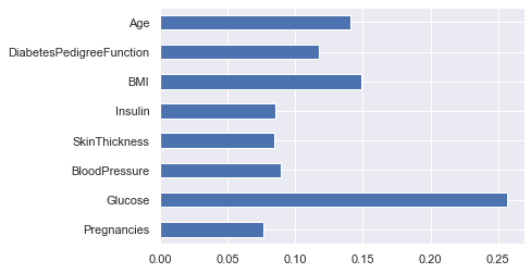
From the graph above, it is clear that ‘Glucose’ is the most essential feature in this dataset. Visualizing feature importance helps us identify which features influence the model’s predictions most.

Saving Model – Random Forest

import pickle 

# Firstly, we will be using the dump() function to save the model using pickle
saved_model = pickle.dumps(rfc) 

# Then we will be loading that saved model
rfc_from_pickle = pickle.loads(saved_model) 

# Lastly, after loading that model we will use this to make predictions 
rfc_from_pickle.predict(X_test)

Output:

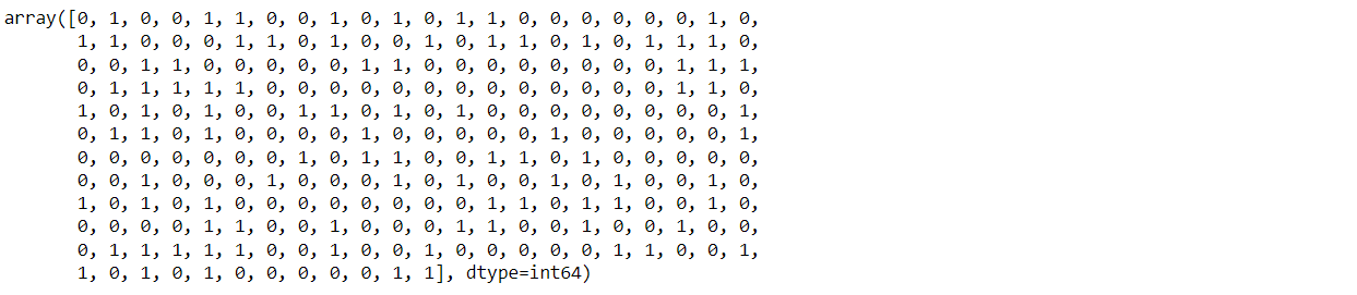
Now, for the last time, I’ll be looking at the dataset’s head and tail so that we can take any random set of features from both to test whether our model is good enough to give the correct prediction.

diabetes_df.head()

Output:

diabetes_df.tail()

Output:

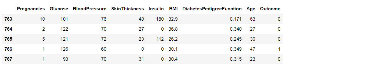
Adding data points to the model will either return 0 or 1, i.e., a person with diabetes or not.

rfc.predict([[0, 137, 40, 35, 168, 43.1, 2.228, 33]]) # 4th patient

Output:

array([1], dtype=int64)

According to our model, this patient has diabetes.

Another one:

rfc.predict([[10, 101, 76, 48, 180, 32.9, 0.171, 63]]) # 763rd patient

Output:

array([0], dtype=int64)

This patient does not have diabetes.

How Can Machine Learning Predict Diabetes?

Data gathering: Collect a thorough dataset detailing individuals’ health records, daily routines, and physical measurements for predicting diabetes through machine learning.

Data preprocessing involves eliminating inconsistencies and errors to clean the data. This measure guarantees the dataset’s appropriateness for training machine learning algorithms in detecting diabetes through machine learning techniques.

Feature Selection: Recognize and choose important attributes like blood sugar levels, BMI, family history, and age. These characteristics are essential for accurately predicting diabetes.

Train models with machine learning algorithms, Such as random forest or neural networks, using the prepared dataset for model training. While being trained, the models are taught to identify patterns that suggest the presence of diabetes by studying examples.

Evaluate the trained models: Performance using accuracy, precision, recall, and F1-score metrics. This measure guarantees the accuracy of diabetes prediction by the models.

Prediction of diabetes: Utilize the trained machine learning models to forecast the probability of individuals experiencing diabetes according to the data provided.

Continuous Monitoring: Set up a mechanism to continuously monitor and revise the models with the arrival of new data. This guarantees that the models stay precise and applicable for forecasting diabetes with machine learning in actual situations.

Alternative Methods for Predicting Diabetes

While machine learning models are highly effective for predicting diabetes, several alternative approaches and models for healthcare can also be used, each with advantages and limitations. Here are some of the leading alternative models for heart disease prediction:

1. Logistic Regression

It is a traditional statistical method used for binary classification problems.

• Advantages: Easy to interpret, requires less computational power, and performs well on smaller datasets.
• Limitations: It may not capture complex relationships and interactions between variables as effectively as machine learning models.

2. Naive Bayes

It is a probabilistic classifier based on Bayes’ theorem with an assumption of independence among predictors.

• Advantages: Simple to implement, performs well with small datasets and high-dimensional data.
• Limitations: Assumes independence among features, which is often unrealistic.

3. K-Nearest Neighbors (KNN)

It is a non-parametric method that classifies a data point based on the majority class of its k nearest neighbors.

• Advantages: Simple to implement and understand, no training phase.
• Limitations: Computationally expensive with large datasets, sensitive to the choice of k and the distance metric.
  

Conclusion

Machine learning offers powerful techniques for disease prediction in healthcare by analyzing various health indicators and lifestyle factors. This comprehensive analysis explored several machine learning algorithms, such as random forests, decision trees, XGBoost, and support vector machines, for building effective diabetes prediction models.

The random forest model emerged as the top performer, achieving an accuracy of 0.77 on the test dataset. We also gained valuable insights into feature importance, with glucose levels being the most influential predictor of diabetes in this dataset. Visualizing the data distributions, correlations, and outliers further enhanced our understanding.

While machine learning excels at diabetes prediction, we discussed alternative methods like logistic regression, naive Bayes, and k-nearest neighbors, each with strengths and limitations. Selecting the right approach depends on factors like dataset size, model interpretability needs, and the complexity of the underlying relationships.

Looking ahead, continued research integrating more extensive and more diverse patient datasets and exploring advanced neural network architectures holds immense potential for improving diabetes prediction accuracy. Additionally, deploying these predictive models in clinical settings can facilitate early intervention, risk stratification, and tailored treatment plans, ultimately improving outcomes for individuals at risk of developing diabetes.

Here’s the repo link to this article.

Here, you can access my other articles, which are published on Analytics Vidhya as a part of the Blogathon (link)

If you want to learn more about artificial intelligence, machine learning, deep learning etc, don’t forget to follow Analytics Vidhya’s blogs.

The media shown in this article is not owned by Analytics Vidhya and is used at the Author’s discretion. 

Frequently Asked Questions

The media shown in this article is not owned by Analytics Vidhya and are used at the Author’s discretion. 

Aman Preet Gulati 25 May 2024