Neural Networks and Deep Learning with Python

This article was published as a part of the Data Science Blogathon.

Introduction

A Neural Network is analogous to the connections of neurons in our brain. In this article, we will see how to set up Neural Networks, Artificial Neural Networks, and Deep Neural Networks, and also how to design the model, how to train it, and finally how to use it for testing. Now we will see how to implement these using Python.

Before going into that, let us talk about Deep Learning and Neural Networks.

Deep Learning:

Deep Learning is a type of machine learning which is very similar to how humans think and gain knowledge about things. Previously invented algorithms are linear, and deep learning is complex.

Neural Networks:

A Neural Network is an assortment of some unit cells, that are interconnected and transmit signals from one to another cell, and they can learn and make decisions.

Deep Learning is very complex and needs to be simplified and broken into simple algorithms, and this can be made possible through a process called visualization.

Setting Neural Networks:

There are many libraries to set up Neural Networks, in this article we will use TensorFlow, which was developed by Google.

Install Tensorflow

pip install tensorflow

The next step is to import the notebook and main modules from TensorFlow Keras. The code is given below.

from tensorflow.keras import models
from tensorflow.keras import layers
from tensorflow.keras import utils
from tensorflow.keras import backend as K
import matplotlib.pyplot as plt
import shap

Artificial Neural Networks

An ANN has an input and an output and is made up of some layers. Neurons, or nodes, are units that connect inputs through a function. This activated function makes neurons switch off or switch on. The weighted inputs have weights, which are randomly initialized, but during training, they will get optimized like all the machine learning algorithms.

As we discussed before, ANNs are made of layers, which in turn are divided into 3 parts.

1-Input Layer

2-Hidden Layer

3-Output Layer

The explanation is similar to their names.

Input Layer- It transfers the input to the Neural Network.

Hidden Layer- It is like an intermediate junction between the input layer and output layer.

Output Layer- It transfers the output to the Neural Network.

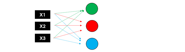
ANNs may have multiple layers with a minimum of 1 layer. ANN with 1 layer is called a perceptron. A perceptron behaves like a simple linear regression model.

Let us go through some examples.

Let us take an example of a dataset having 3 inputs and one output.

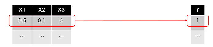
source: https://miro.medium.com/max/700/1*lFLZJTfOovO-XDSXN5Qtbg.png

The common thing we need to do in machine learning models is training.

Training is finding the best parameters so that error is minimized.

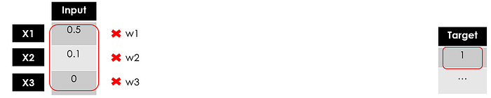                                                                                   Source: https://miro.medium.com/max/700/1*OUSayv9gfDsGfHgoHxjMXQ.png

w1, w2, and w3 are weights that can be initialized randomly. Let us initialize with 1.

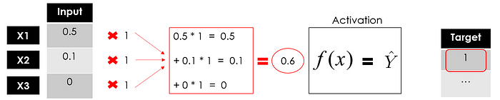
Source: https://miro.medium.com/max/700/1*pYsVp9uCTNvzGrVWaqgbiA.png

Here we used a linear function to determine the output, so it is very much like linear regression.

As we saw, it is a perceptron. It has 3 inputs and one output. In this training, we will compare the output each time with the predicted one, optimize the parameters, or change the function so that it will be close to the expected value.

A Neuron is represented as,

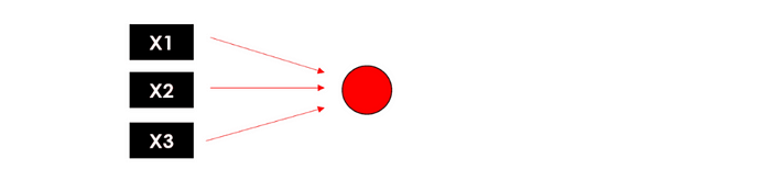                                                             Source: https://miro.medium.com/max/700/1*h4lmqakEKfEvxMoqSFx2yA.png

Deep Neural Networks

A neural network is said to be deep when it has at least 2 hidden layers so that it has 1 input layer, at least 2 hidden layers, and 1 output layer.

In a DNN, the process happens three times simultaneously and sends the output to the first hidden layer, which in turn becomes the input for the second hidden layer.

                                                                        Source: https://miro.medium.com/max/700/1*Y8LQ1EZJKnCt2-u4vwN0Rg.png

The second hidden layer takes the input from the first hidden layer and sends the output to the output layer.

                                                                                 Source: https://miro.medium.com/max/700/1*jCtuDvOx21mYXi2cmdRMSA.gif

Model Design

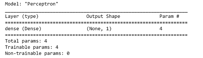
Now we will build a neural network with TensorFlow.

model = models.Sequential(name="Perceptron", layers=[    layers.Dense(      
          name="dense",
          input_dim=3,        
          units=1,            
          activation='linear' #f(x)=x
    )
])
model.summary()

                                                                                       Source: https://miro.medium.com/max/700/1*nke8IcOb3b8xPwBq7tCDcw.png

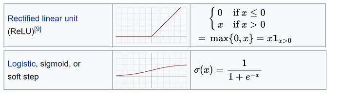
If we want to use a binary function instead of the linear function,

# define the function
import tensorflow as tf

def binary_step_activation(x):

    ##return 1 if x>0 else 0 
    return K.switch(x>0, tf.math.divide(x,x), tf.math.multiply(x,0))
# build the model
model = models.Sequential(name="Perceptron", layers=[
      layers.Dense(             
          name="dense",
          input_dim=3,        
          units=1,            
          activation=binary_step_activation
      )
])

We have discussed perceptron models. Let us go to the DNNs.

We need to know the following parameters before building a deep neural network:

1. Number of Layers

2. Number of neurons

3. Activation function

Number of Neurons = (Number of inputs + 1 output)/2

The activation function depends on the problem. For example, linear functions are used for regression models, and sigmoid functions are used for classification models.

                                                                             Source: https://miro.medium.com/max/700/1*LqUJbrGw6wwyix6atFaSZQ.png

Let us take an example with N inputs and one output.

n_features = 10model = models.Sequential(name="DeepNN", layers=[
    ### hidden layer 1
    layers.Dense(name="h1", input_dim=n_features,
                 units=int(round((n_features+1)/2)), 
                 activation='relu'),
    layers.Dropout(name="drop1", rate=0.2),
    
    ### hidden layer 2
    layers.Dense(name="h2", units=int(round((n_features+1)/4)), 
                 activation='relu'),
    layers.Dropout(name="drop2", rate=0.2),
    
    ### layer output
    layers.Dense(name="output", units=1, activation='sigmoid')
])
model.summary()

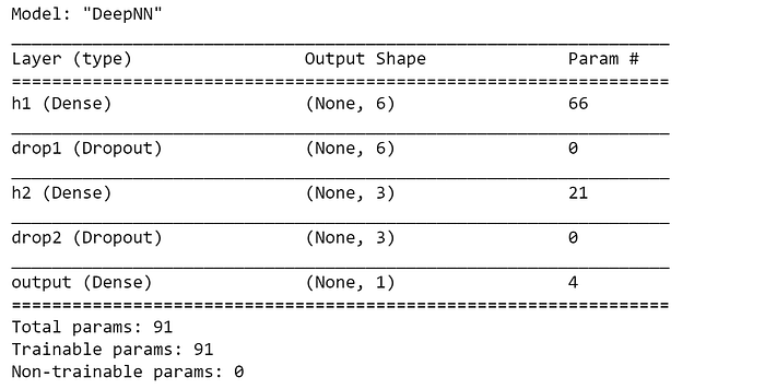
Source:https://miro.medium.com/max/700/1*zVB4XJugIya9yW0tB43qtA.png

Now we are going to use model class to build perceptron.

# Perceptron
inputs = layers.Input(name="input", shape=(3,))
outputs = layers.Dense(name="output", units=1, 
                       activation='linear')(inputs)
model = models.Model(inputs=inputs, outputs=outputs, 
                     name="Perceptron")

Next is using the model class to build a Deep Neural Network.

# DeepNN
### layer input
inputs = layers.Input(name="input", shape=(n_features,))### hidden layer 1
h1 = layers.Dense(name="h1", units=int(round((n_features+1)/2)), activation='relu')(inputs)
h1 = layers.Dropout(name="drop1", rate=0.2)(h1)### hidden layer 2
h2 = layers.Dense(name="h2", units=int(round((n_features+1)/4)), activation='relu')(h1)
h2 = layers.Dropout(name="drop2", rate=0.2)(h2)### layer output
output = layers.Dense(name="output", activation='sigmoid')(h2)
model = models.Model(inputs=inputs, outputs=outputs)

Visualization

The function for plotting an ANN using the TensorFlow model is given below.

def utils_nn_config(model):
    lst_layers = []
    if "Sequential" in str(model): #-> Sequential doesn't show the input layer
        layer = model.layers[0]
        lst_layers.append({"name":"input", "in":int(layer.input.shape[-1]), "neurons":0, 
                           "out":int(layer.input.shape[-1]), "activation":None,
                           "params":0, "bias":0})
    for layer in model.layers:
        try:
            dic_layer = {"name":layer.name, "in":int(layer.input.shape[-1]), "neurons":layer.units, 
                         "out":int(layer.output.shape[-1]), "activation":layer.get_config()["activation"],
                         "params":layer.get_weights()[0], "bias":layer.get_weights()[1]}
        except:
            dic_layer = {"name":layer.name, "in":int(layer.input.shape[-1]), "neurons":0, 
                         "out":int(layer.output.shape[-1]), "activation":None,
                         "params":0, "bias":0}
        lst_layers.append(dic_layer)
    return lst_layers

def visualize_nn(model, description=False, figsize=(10,8)):

    lst_layers = utils_nn_config(model)
    layer_sizes = [layer["out"] for layer in lst_layers]
   
    fig = plt.figure(figsize=figsize)
    ax = fig.gca()
    ax.set(title=model.name)
    ax.axis('off')
    left, right, bottom, top = 0.1, 0.9, 0.1, 0.9
    x_space = (right-left) / float(len(layer_sizes)-1)
    y_space = (top-bottom) / float(max(layer_sizes))
    p = 0.025
    ## nodes
    for i,n in enumerate(layer_sizes):
        top_on_layer = y_space*(n-1)/2.0 + (top+bottom)/2.0
        layer = lst_layers[i]
        colour = "green" if i in [0, len(layer_sizes)-1] else "blue"
        colour = "red" if (layer['neurons'] == 0) and (i > 0) else color
        ### add description
        if (description is True):
            d = i if i == 0 else i-0.5
            if layer['activation'] is None:
                plt.text(x=left+d*x_space, y=top, fontsize=10, color=color, s=layer["name"].upper())
            else:
                plt.text(x=left+d*x_space, y=top, fontsize=10, color=color, s=layer["name"].upper())
                plt.text(x=left+d*x_space, y=top-p, fontsize=10, color=color, s=layer['activation']+" (")
                plt.text(x=left+d*x_space, y=top-2*p, fontsize=10, color=color, s="Σ"+str(layer['in'])+"[X*w]+b")
                out = " Y"  if i == len(layer_sizes)-1 else " out"
                plt.text(x=left+d*x_space, y=top-3*p, fontsize=10, color=color, s=") = "+str(layer['neurons'])+out)
        ### circles
        for m in range(n):
            color = "limegreen" if color == "green" else color
            circle = plt.Circle(xy=(left+i*x_space, top_on_layer-m*y_space-4*p), radius=y_space/4.0, color=color, ec='k', zorder=4)
            ax.add_artist(circle)
            ### add text
            if i == 0:
                plt.text(x=left-4*p, y=top_on_layer-m*y_space-4*p, fontsize=10, s=r'$X_{'+str(m+1)+'}$')
            elif i == len(layer_sizes)-1:
                plt.text(x=right+4*p, y=top_on_layer-m*y_space-4*p, fontsize=10, s=r'$y_{'+str(m+1)+'}$')
            else:
                plt.text(x=left+i*x_space+p, y=top_on_layer-m*y_space+(y_space/8.+0.01*y_space)-4*p, fontsize=10, s=r'$H_{'+str(m+1)+'}$')
    ## links
    for i, (n_a, n_b) in enumerate(zip(layer_sizes[:-1], layer_sizes[1:])):
        layer = lst_layers[i+1]
        color = "green" if i == len(layer_sizes)-2 else "blue"
        color = "red" if layer['neurons'] == 0 else color
        layer_top_a = y_space*(n_a-1)/2. + (top+bottom)/2. -4*p
        layer_top_b = y_space*(n_b-1)/2. + (top+bottom)/2. -4*p
        for m in range(n_a):
            for o in range(n_b):
                line = plt.Line2D([i*x_space+left, (i+1)*x_space+left], 
                                  [layer_top_a-m*y_space, layer_top_b-o*y_space], 
                                  c=color, alpha=0.5)
                if layer['activation'] is None:
                    if o == m:
                        ax.add_artist(line)
                else:
                    ax.add_artist(line)
    plt.show()

visualize_nn(model, description=True, figsize=(10,8))

We are going to visualize our perceptron model and DNN model.

First, we will see the perceptron model.

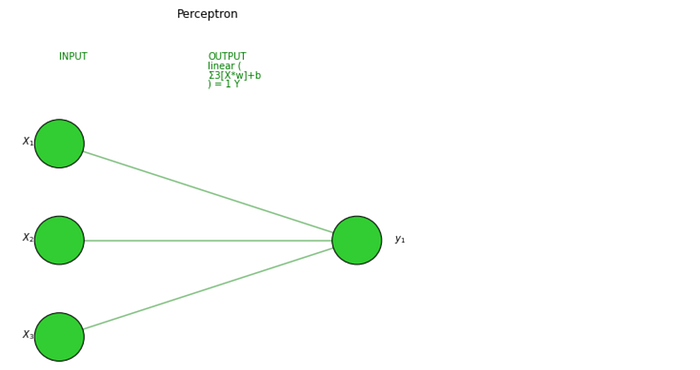
Source: https://miro.medium.com/max/700/1*EQ-X0B264W2JZzXaMO2P_w.png

The below image is for a Deep Neural Network.

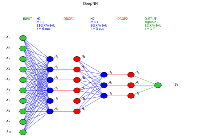
Source: https://miro.medium.com/max/700/1*ApgZUAinNP5cvcPyfrs84g.png

utils.plot_model(model, to_file='model.png', show_shapes=True, show_layer_names=True)

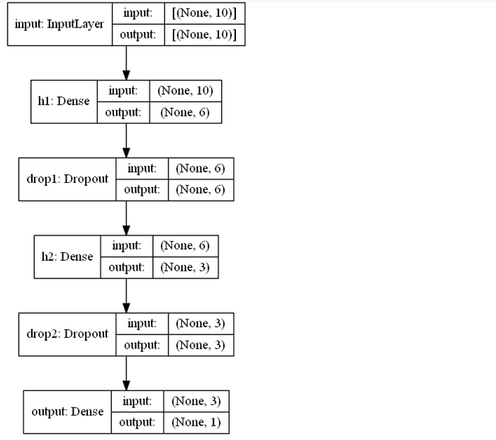                                                      Source: https://miro.medium.com/max/700/1*xqsAhVdEdmR3IIi0fvLarA.png

Training and Testing

We need an optimizer, a loss function, and metrics. We can use Adam Optimizer.

# define metrics
def Recall(y_true, y_pred):
    true_positives = K.sum(K.round(K.clip(y_true * y_pred, 0, 1)))
    possible_positives = K.sum(K.round(K.clip(y_true, 0, 1)))
    recall = true_positives / (possible_positives + K.epsilon())
    return recall

def Precision(y_true, y_pred):
    true_positives = K.sum(K.round(K.clip(y_true * y_pred, 0, 1)))
    predicted_positives = K.sum(K.round(K.clip(y_pred, 0, 1)))
    precision = true_positives / (predicted_positives + K.epsilon())
    return precision

def F1(y_true, y_pred):
    precision = Precision(y_true, y_pred)
    recall = Recall(y_true, y_pred)
    return 2*((precision*recall)/(precision+recall+K.epsilon()))

model.compile(optimizer='adam', loss='binary_crossentropy', 
              metrics=['accuracy',F1])

# define metrics
def R2(y, y_hat):
    ss_res =  K.sum(K.square(y - y_hat)) 
    ss_tot = K.sum(K.square(y - K.mean(y))) 
    return ( 1 - ss_res/(ss_tot + K.epsilon()) )

model.compile(optimizer='adam', loss='mean_absolute_error', 
              metrics=[R2])

During training, we can find that accuracy increases and loss decreases. We will keep some data sets for testing.

If we don’t have our data ready, we can generate random data using the following code.

import numpy as np

X = np.random.rand(1000,10)
y = np.random.choice([1,0], size=1000)

# train/validation
training = model.fit(x=X, y=y, batch_size=30, epochs=100, shuffle=True)
       
## training    
ax[0].set(title="Training")    
ax11 = ax[0].twinx()    
ax[0].plot(training.history['loss'], color='black')    ax[0].set_xlabel('Epochs')    
ax[0].set_ylabel('Loss', color='black')    
for metric in metrics:        
    ax11.plot(training.history[metric], label=metric)    ax11.set_ylabel("Score", color='steelblue')    
ax11.legend()
        
## validation    
ax[1].set(title="Validation")    
ax22 = ax[1].twinx()    
ax[1].plot(training.history['val_loss'], color='black')    ax[1].set_xlabel('Epochs')    
ax[1].set_ylabel('Loss', color='black')    
for metric in metrics:          
    ax22.plot(training.history['val_'+metric], label=metric)    ax22.set_ylabel("Score", color="steelblue")    
plt.show()

For Classification example,

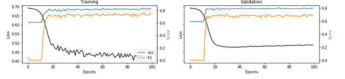                                                                              Source: https://miro.medium.com/max/700/1*lu3vNfJiREvKtBRuVkI2tg.png

For Regression example,

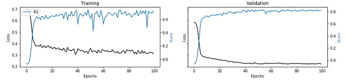                                                                                 Source: https://miro.medium.com/max/700/1*FTjn3ceF-sXjs9ljK0D5NQ.png

Now coming to the testing part,

i = 1explainer_shap(model,

               X_names=list_feature_names, 
               X_instance=X[i], 
               X_train=X, 
               task="classification", #task="regression"
               top=10)

                                 Source: https://miro.medium.com/max/700/1*FxIkl_wUXQA8lJ0OP2ziQA.png

Conclusion on Neural Networks

Neural networks are quite famous these days. These are majorly used in computer vision tasks, from speech recognition to pattern recognition and solving problems. In the future, these will replace human labour. Deep Learning Neural Networks work not only based on the algorithms but also on previous experiences. Overall, in this article, we have seen

–> About Deep Learning and Neural Networks

–> How to Set Up Neural Networks, Artificial Neural Networks, and Deep Neural Networks

–> How to design the model

–> Visualization part

–> Finally, Training and Testing

Hope you guys found it useful.

Connect with me on LinkedIn.

Thanks!

The media shown in this article is not owned by Analytics Vidhya and is used at the Author’s discretion.