Building a Deep Learning Image Classifier with Keras using R

This article was published as a part of the Data Science Blogathon.

Introduction

An important application of deep learning and artificial intelligence is image classification. Image classification is the process of labeling images based on specific characteristics or features that they contain. The algorithm recognizes these qualities and utilizes them to distinguish between images and assign labels to them. Convolutional neural networks (CNNs) are the primary building blocks of deep learning image classification models. These are often used for image recognition, image classification, object detection, and other similar tasks.

Python is widely used for image classification problems. TensorFlow and Keras are two popular packages used for building image classifiers in Python. However, these two libraries can also be used in an R environment. This article explains a step-by-step approach to building a deep learning image classifier model with Keras in R.

MNIST Fashion Image Classifier

We will build an image classifier that can classify apparel images such as dresses, shirts, and jackets.

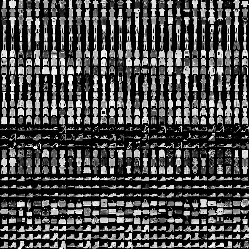
We will be using the Fashion MNIST dataset, which has 70,000 grayscale images. Each image is a grayscale 28 x 28 image classified into 10 separate categories. Each image has a label attached to it. There are ten labels in total:

• T-shirt/top
• Trouser
• Pullover
• Dress
• Coat
• Sandal
• Shirt
• Sneaker
• Bag
• Ankle boot

Let’s import all the required libraries first.

library(keras)
library(tidyverse)

The Fashion MNIST dataset is then directly imported from Keras using the below commands. In addition, 60,000 images will be used to train the model, and 10,000 images will be used to evaluate how well the model learned to classify images.

fashion_mnist <- dataset_fashion_mnist()
c(train_images, train_labels) %<-% fashion_mnist$train
c(test_images, test_labels) %<-% fashion_mnist$test

We now have four arrays: The train_images and train_labels arrays contain the training set, which is the data used by the model to train. The model is validated against the test set, including the test_images and test_label arrays. Each image is a 28 x 28 array with pixel values ranging from 0 to 255. The labels are integer arrays ranging from 0 to 9. These relate to the class of clothes. Following that, a single label is assigned to each image. Because the class names are not included in the dataset, we’ll save them in a vector using the following command and utilize them later when plotting the images.

class_names = c('T-shirt/top',
                'Trouser',
                'Pullover',
                'Dress',
                'Coat', 
                'Sandal',
                'Shirt',
                'Sneaker',
                'Bag',
                'Ankle boot')

Before we train the model, let’s look at the dataset’s format. Using the commands below, we will print the dimensions of train images and train labels, which are 60,000 images with 28 × 28 pixels each.

dim(train_images)

dim(train_labels)

Similarly, the dimensions of test images and test labels, 10,000 images each with a size of 28 x 28 pixels, are printed using the commands below.

dim(test_images)

dim(test_labels)

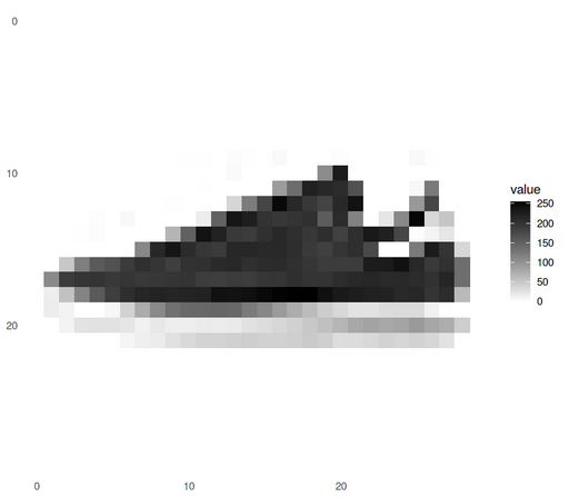
Then, we’ll use the following command to view a sample image from the dataset.

options(repr.plot.width=7, repr.plot.height=7) 
sample_image <- as.data.frame(train_images[7, , ])
colnames(sample_image) <- seq_len(ncol(sample_image))
sample_image$y <- seq_len(nrow(sample_image))
sample_image <- gather(sample_image, "x", "value", -y)
sample_image$x <- as.integer(sample_image$x)
ggplot(sample_image, aes(x = x, y = y, fill = value)) +
    geom_tile() + scale_fill_gradient(low = "white", high = "black", na.value = NA) +
    scale_y_reverse() + theme_minimal() + theme(panel.grid = element_blank()) +
    theme(aspect.ratio = 1) + xlab("") + ylab("")

Before training the model, the data must be pre-processed. To reduce the pixel values, we must normalize the data. Currently, all image pixels have values ranging from 0-255, and we want values between 0 and 1. As a result, we will divide all the pixel values into the train and test sets by 255.0.

train_images <- train_images / 255
test_images <- test_images / 255

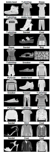
To ensure that the data is in the right format, let us view the first 30 images from the training set. We will also display the class name below each image.

options(repr.plot.width=10, repr.plot.height=10)
par(mfcol=c(10,10))
par(mar=c(0, 0, 1.5, 0), xaxs='i', yaxs='i')
for (i in 1:30) { 
  img <- train_images[i, , ]
  img <- t(apply(img, 2, rev)) 
  image(1:28, 1:28, img, col = gray((0:255)/255), xaxt = 'n', yaxt = 'n',
        main = paste(class_names[train_labels[i] + 1]))}

Now it’s time to build our model.

Building the Model

To build a neural network, we require configuring the layers of the model as follows –

1. Convolution or Conv2D Layer: A convolution layer extracts features from an image or a part of an image. We are specifying three parameters here:

• Filters – This is the number of filters that will be used in the convolution. E.g., 32 or 64.
• Kernel size – The length of the convolution window. E.g. (3,3) or (4,4).
• Activation – This refers to the function of the regularizer. For example, ReLU, Leaky ReLU, Tanh, and Sigmoid.

2. Pooling or MaxPooling2D Layer: This layer is used to reduce the size of an image.

3. Flatten Layer: This layer reduces an n-dimensional array to a single dimension.

4. Dense Layer: This layer is fully connected, which means that all of the neurons in the present layer are linked to the next layer. For our model, we have 128 neurons in the first dense layer and 10 neurons in the second dense layer.

5. Dropout Layer: To prevent the model from overfitting, this layer ignores a set of neurons (randomly).

model <- keras_model_sequential()
model %>%
    layer_conv_2d(filters = 32, kernel_size = c(3,3), 
                   activation = 'relu', input_shape = c(28, 28, 1)) %>%
    layer_max_pooling_2d(pool_size = c(2,2)) %>%
    layer_flatten() %>%
    layer_dense(units = 128, activation = 'relu') %>%
    layer_dropout(rate = 0.5) %>%
    layer_dense(units = 10, activation = 'softmax')

A few additional settings are required before the model is ready for training. These are added at the compile step of the model:

1. Loss function – This function evaluates how effectively our algorithm represents the dataset. Depending on our dataset, we can choose from alternatives such as ‘categorical_cross_entropy,’ ‘binary_cross_entropy,’ and ‘sparse categorical_cross_entropy.’

2. Optimizer – With this, we can adjust a neural network’s weights and learning rate. We can select from many optimizers such as Adam, AdaDelta, SGD, and others.

3. Metrics – These are used to evaluate the performance of our model. For example, accuracy, mean squared error, etc.

model %>% compile(
    loss = 'sparse_categorical_crossentropy',
    optimizer = 'adam', 
    metrics = c('accuracy')
)

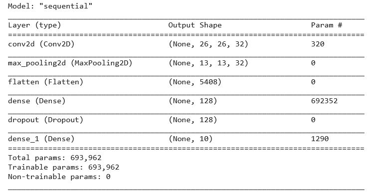
All the parameters and shapes in our model’s layers can be seen using the ‘summary’ function as shown below.

summary(model)

To begin training, we will call the fit method, which will use the training and test data as well as the following inputs to fit our model:

history % fit(x_train, train_labels, epochs = 20,verbose=2)

1. Epochs – The number of times the entire dataset is sent forward and backward through the neural network.
2. Verbose – Viewing choices for our output. For example, verbose = 0 prints nothing, verbose = 1 prints the progress bar and one line every epoch, and verbose = 2 prints one line each epoch.

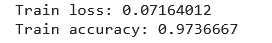
After running the model with 20 Epochs, we are getting 97.36% training accuracy.

score % evaluate(x_train, train_labels)
cat('Train loss:', score$loss, "n")
cat('Train accuracy:', score$acc, "n")

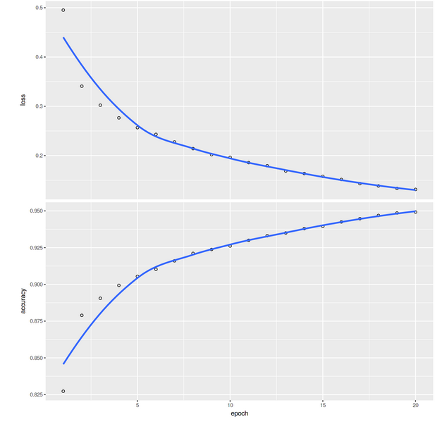
We can plot the accuracy-loss graph along with the epochs using the following command:

plot(history)

Now we will see how the model performs on the test dataset:

score % evaluate(x_test, test_labels)
cat('Test loss:', score$loss, "n")
cat('Test accuracy:', score$acc, "n")

We are getting an accuracy of 91.6% on the test dataset. We can utilize the trained model to make predictions on some test images.

predictions % predict(x_test)

We got the predictions from the model, i.e., a label for each image in the test set. Let’s look at the first prediction:

predictions[1, ]

A prediction is a set of ten numbers. These express the model’s “confidence” that the images represent each of the 10 items of clothing.

As an alternative, we can also print the class prediction directly using the following command:

class_pred % predict_classes(x_test)
class_pred[1:20]

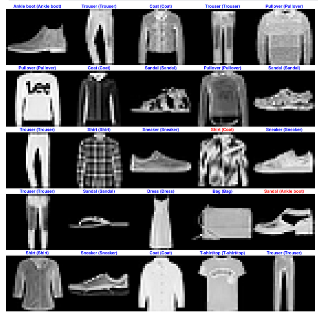
Now we will plot a few images with their predictions. Correct predictions are in blue, whereas wrong predictions are in red.

options(repr.plot.width=7, repr.plot.height=7)
par(mfcol=c(5,5))
par(mar=c(0, 0, 1.5, 0), xaxs='i', yaxs='i')
for (i in 1:25) { 
  img <- test_images[i, , ]
  img <- t(apply(img, 2, rev)) 
  predicted_label <- which.max(predictions[i, ]) - 1
  true_label <- test_labels[i]
  if (predicted_label == true_label) { color <- 'blue' } 
    else 
    { color <- 'red' }
  image(1:28, 1:28, img, col = gray((0:255)/255), xaxt = 'n', yaxt = 'n',
        main = paste0(class_names[predicted_label + 1], 
                       "(",class_names[true_label + 1], ")"),col.main = color)}

That’s how you can use Keras for image classification in R!

Conclusion

In this article, we learned how to build a deep learning image classifier with Keras in R. The model is highly accurate on the test data. However, it is essential to remember that the accuracy can change depending on the training set. Thus, the model will not work with images appearing different than the ones it was trained on.

Here are some key takeaways from this article-

• Both Tensorflow and Keras have official R support.
• It was easy to set up and train the model in R, just like Python.
• The approach in this article can be applied to another image dataset for classification, or the trained model can be saved and deployed as an app.

I hope you enjoyed building this deep learning image classifier in R. The code for this tutorial is available on my GitHub repository.

The media shown in this article is not owned by Analytics Vidhya and is used at the Author’s discretion.