How to Make an Image Classification Model Using Deep Learning?
This article was published as a part of the Data Science Blogathon.
Introduction
In the 21st century, the world is rapidly moving towards Artificial Intelligence and Machine Learning. Various robust AI Models have been made that perform far better than the human brain, like deepfake generation, image classification, text classification, etc. Companies are investing vast amounts of money to make these models, so there is a suitable time for a person who wants to start exploring their career in this field.
Therefore, I will show you how you can make a simple image classification model using a Convolutional Neural Network in this article. We will classify the images of cats and dogs. It is a perfect problem statement to work with at an elementary level. After training our model, we will also optimize its performance by applying various optimization techniques, which I will discuss later in this article.
There are various applications of Image Classification like Computer Vision, Traffic Control systems, Brake Light Detection, Detection of diseases, etc. And the basis for Image classification is Convolutional Neural Network(CNN), so let us talk first about it.
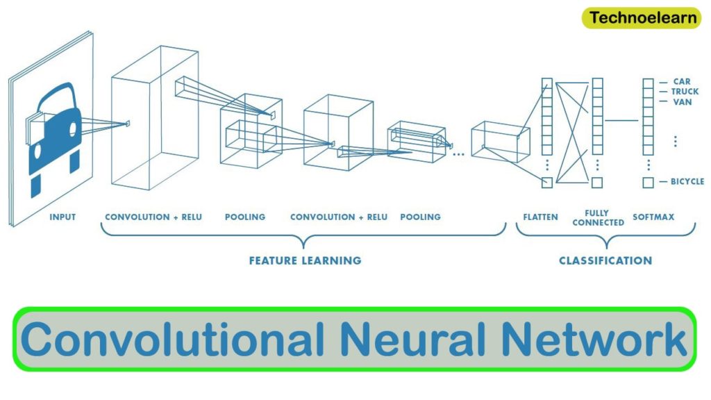
What is CNN in Image Classification?
Convolutional Neural Networks, often known as CNNs, are a subset of artificial neural networks used in deep learning and are frequently employed for object and picture identification and categorization. Thus, Deep Learning utilizes a CNN to identify items in a picture.
CNN is a deep learning model to process data with a grid pattern, such as images. CNN was inspired by how the animal visual cortex is organized [13, 14] and is intended to automatically and adaptively learn spatial hierarchies of features, from low- to high-level patterns.
Code Implementation
In this section, we will discuss code implementation. Firstly we will import all the necessary libraries. After this, we will load and pre-process the dataset. Then after it, we will train the CNN model and calculate its accuracy on the test set.
Finally, we will apply different optimization techniques to it, discussed above, and compare the best among them.
Importing necessary libraries:
We will import all the required libraries like Numpy, Pandas, Torchvision, Keras, etc. Popular datasets, model architectures, and typical image modifications for computer vision are all included in the torchvision package.
import torchvision.transforms as transforms

import torchvision.datasets as datasets

import torchvision.models as models

import torch.nn as nn

import torch.optim as optim

import numpy as np

from PIL import Image

import numpy as np
import matplotlib
from torchvision.datasets import ImageFolder
from torch.utils.data import DataLoader

from imutils import paths import shutil
Loading Dataset:
We have used the cats and dog dataset, which contains several images of cats and dogs. You can download that using this link.
This dataset contains 12501 images of cats and dogs each.
The function named below copy_images is used to extract the images from the directory and read them to put in an array using open cv libraries.
After that, we will resize the images and perform horizontal and vertical flipping. It gives some more about the robustness of our model.
Finally, we will divide this dataset into the train, test, and validation sets.
neg_num, negs_num = -1, -2

import os

def copy_images(imagePaths, folder):

if not os.path.exists(folder):

os.makedirs(folder)

for path in imagePaths:

zer = 0

v = zer

try:

img = matplotlib.image.mpimg.imread(path)

except:

print("found1 ",path,"n")

else:

one_num =1

v = one_num

if v == one_num:

imageName = path.split(os.path.sep)[neg_num]

label = path.split(os.path.sep)[negs_num]

ing, ing1 = folder, label

labelFolder = os.path.join(ing, ing1)

if not os.path.exists(labelFolder):

os.makedirs(labelFolder)

destination = os.path.join(labelFolder, imageName)

cp, dest = path, destination
shutil.copy(cp, dest)
resize = transforms.Resize(size=(INPUT_HEIGHT,INPUT_WIDTH))

hFlip = transforms.RandomHorizontalFlip(p=0.25)
trainTransforms, testTransforms = transforms.Compose([resize,transforms.ToTensor()]), transforms.Compose([resize,transforms.ToTensor()])
imagePaths = list(paths.list_images("PetImages"))

np.random.shuffle(imagePaths)

num, num1 = 0.3, 0.07

val, val1 = len(imagePaths) * num, len(imagePaths) * num1

testPathsLen,valPathsLen = int(val), int(val1)

trainPathsLen = len(imagePaths) - valPathsLen - testPathsLen

trainPaths,valPaths,testPaths = imagePaths[:trainPathsLen], imagePaths[trainPathsLen:trainPathsLen+valPathsLen+1], imagePaths[trainPathsLen+valPathsLen+1:]

copy_images(trainPaths, "train")

copy_images(valPaths, "val")

copy_images(testPaths, "test")
Data Visualization:
Now, we will print random images of both classes to visualising the data better. It helps us to find the right and perfect algorithm to train our model.
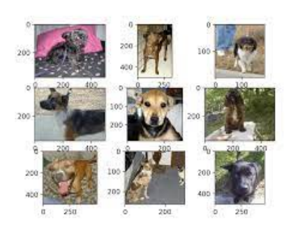
We will make a function named “visualize_batch,” which reads some random images one by one and plots them in a map using the matplotlib library.
After that, we will use a Data Loader to visualize the train, test, and validation sets separately.
def visualize_batch(batch, classes, dataset_type):

val = 32

hund = 100

fig = matplotlib.pyplot.figure("{} batch".format(dataset_type),

figsize=(val, val))

for i in range(0, hund):

ghr, ytu = 25,4

ax = matplotlib.pyplot.subplot(ghr, ytu, i + 1)

image = batch[0][i].cpu().numpy()

if(np.all((image == 0.0))):

print("iszero")

one, two, zer = 1,2,0

image = image.transpose((one, two, zer))

image = (image * 255.0).astype("uint8")

idx = batch[one][i]

label = classes[idx]

print(idx,label)

matplotlib.pyplot.imshow(image)

matplotlib.pyplot.title(label)

matplotlib.pyplot.axis("off")

matplotlib.pyplot.tight_layout()
matplotlib.pyplot.show()
# initialize the training and validation dataset

trainDataset, testDataset, valDataset = ImageFolder(root="train", transform=trainTransforms), ImageFolder(root="test", transform=testTransforms), ImageFolder(root="val", transform=testTransforms)
trainDataLoader,valDataLoader,testDataLoader = DataLoader(trainDataset,batch_size=BATCH_SIZE, shuffle=True), DataLoader(dataset = valDataset, batch_size=BATCH_SIZE, shuffle=True), DataLoader(testDataset, batch_size=BATCH_SIZE, shuffle=True)
from PIL import Image
trainBatch, testBatch,valBatch = next(iter(trainDataLoader)), next(iter(testDataLoader)), next(iter(valDataLoader))
visualize_batch(trainBatch, trainDataset.classes, "train")
Checking the availability of Cuda Cores:
Check if your machine contains a GPU or not. A GPU is a Graphic Processing Unit that is specially designed hardware that accelerates the rendering of an image and its processing. Using a GPU will fasten your training process.
The below code will shift your runtime from CPU to GPU if you have CUDA Cores available.
device = 'cuda' if torch.cuda.is_available() else 'cpu'
Training CNN Model:
Now we will make a three-layered convolutional neural network to train our model. This model contains Conv2D layers, Max Pooling layers, Flattening layers, Dropout layers, etc.
Our 1st layer contains a Conv2D layer of size 32×32 and a Max Pooling layer of strides 2. It is similar for layer2 and layer3, but the size of conv2D layers are different, which you can check in the code itself.
After applying the Convolutional layers, now we will use a flattening layer to convert the 2D array to a 1D array. Then we will apply a combination of dense and dropout layers to obtain the final classification.
At last, the function named “test_accuracy” is used to evaluate our trained model’s accuracy and precision scores on the test set.
ks = 3
pads = 0
neg_one =1
strides = 2
var, var1, var2 = 32,64,128
drop_ratio = 0.5
num2 = 10
class Cnn(nn.Module):
    def __init__(self):
        super(Cnn,self).__init__()

        self.layer1 = nn.Sequential(
            nn.Conv2d(3,var,kernel_size=ks, padding=pads,stride=strides),
            nn.MaxPool2d(strides)
            nn.ReLU()

        )

        self.layer2 = nn.Sequential(
            nn.Conv2d(var, var1, kernel_size=ks, padding=pads, stride=strides),
            nn.MaxPool2d(strides)
            nn.ReLU()
            )

        self.layer3 = nn.Sequential(
            nn.Conv2d(var1, var2, kernel_size=ks, padding=pads, stride=strides),
            nn.MaxPool2d(strides)
            nn.ReLU()
        )

        self.fc1 = nn.Linear(3*3*128,num2)
        self.dropout = nn.Dropout(drop_ratio)
        self.fc2 = nn.Linear(num2,strides)
        self.relu = nn.ReLU()
        self.sigmoid = nn.sigmoid()


    def forward(self,x):
        out = self.layer1(x)
        out = self.layer2(out)
        out = self.layer3(out)
        out = out.view(out.size(pads),neg_one)
        out = self.relu(self.fc1(out))
        out = self.fc2(out)
        out = self.sigmoid(out)
        return out

model = Cnn().to(device)
model.train()

def test_accuracy(loader,model):
    num_correct,num_samples  = 0, 0
    model.eval()

    with torch.no_grad():
        for x, y in loader:
            x, y = x.to(device=device), y.to(device=device)
            scores = model(x)
            acc = (scores.argmax(dim = 1) == y).sum()
            num_correct = num_correct+acc
            num_samples = num_samples+y.size(0)

        print(f'Got {num_correct} / {num_samples} with accuracy {float(num_correct)/float(num_samples)*200:.2f}')

    model.train()
Applying Optimizations
In this section, we will apply several optimizations like Vanilla SGD Optimizer, Minibatch with SGD Optimizer, etc., to further increase the accuracy and precision of our previously trained model.
We train the model iteratively through optimization, which assesses the maximum and minimum functions. One of the most significant phenomena in machine learning is the desire for improved outcomes.
1. Vanilla SGD:
It wouldn’t be pure gradient descent because it is a variation of the standard gradient descent. In contrast to more elaborate SGD options, such as SGD with momentum, this may be referred to as “vanilla stochastic gradient descent” because even stochastic gradient descent has several variations.
We make empty lists for validation losses, training losses, and accuracy. After that, we will apply optim.SGD function with CrossEntropyLoss(), and give the complete model as parameters to optimize it.
val_losses, val_acc, train_losses, train_acc = list(), list(),list(),list()


lr_val = 0.01

optimizer2 = optim.SGD(params = model.parameters(),lr=lr_val)

criterion2 = nn.CrossEntropyLoss()


bs, rt = 100, False

trainDataLoader, valDataLoader, testDataLoader = DataLoader(trainDataset,batch_size=bs, shuffle=rt), DataLoader(dataset = valDataset, batch_size=bs, shuffle=rt), DataLoader(testDataset, batch_size=bs, shuffle=rt)

trainer(model,trainDataLoader,valDataLoader,testDataLoader,optimizer2,criterion2,val_losses,val_acc,train_losses,train_acc)
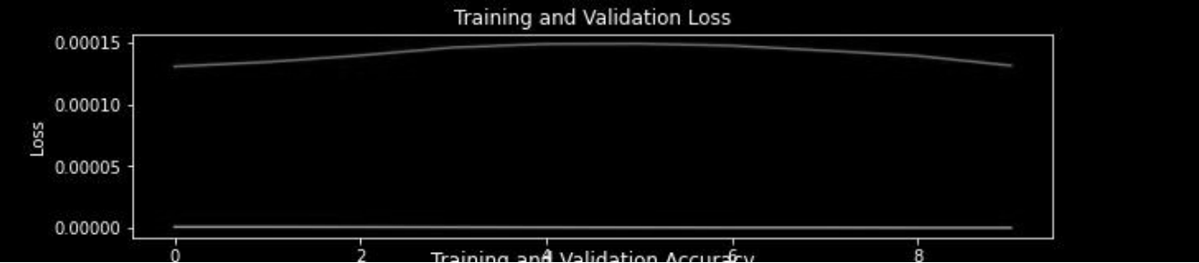
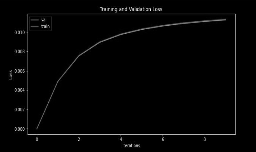
Loss curve:
In this curve, we have seen that both training and validation loss remains constant as we increase the number of iterations or epochs.
We will use the matplotlib library to plot the loss graph.
matplotlib.pyplot.figure(figsize=(10,5))

matplotlib.pyplot.title("Training and Validation Loss")

matplotlib.pyplot.plot(val_losses,label="Val")

matplotlib.pyplot.plot(train_losses,label="train")

matplotlib.pyplot.xlabel("iterations")

matplotlib.pyplot.ylabel("Loss")

matplotlib.pyplot.legend()

matplotlib.pyplot.show(
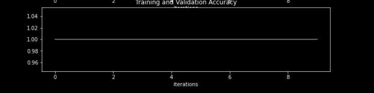
Accuracy Curve:
In this curve, we have seen that both training and validation accuracy remains constant as we increase the number of iterations or epochs.
matplotlib.pyplot.figure(figsize=(10,5))

matplotlib.pyplot.title("Training and Validation Accuracy")

matplotlib.pyplot.plot(val_losses,label="Val")

matplotlib.pyplot.plot(train_losses,label="train")

matplotlib.pyplot.xlabel("iterations")

matplotlib.pyplot.ylabel("accuracy")

matplotlib.pyplot.legend()

matplotlib.pyplot.show()
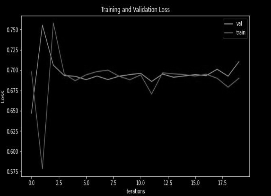
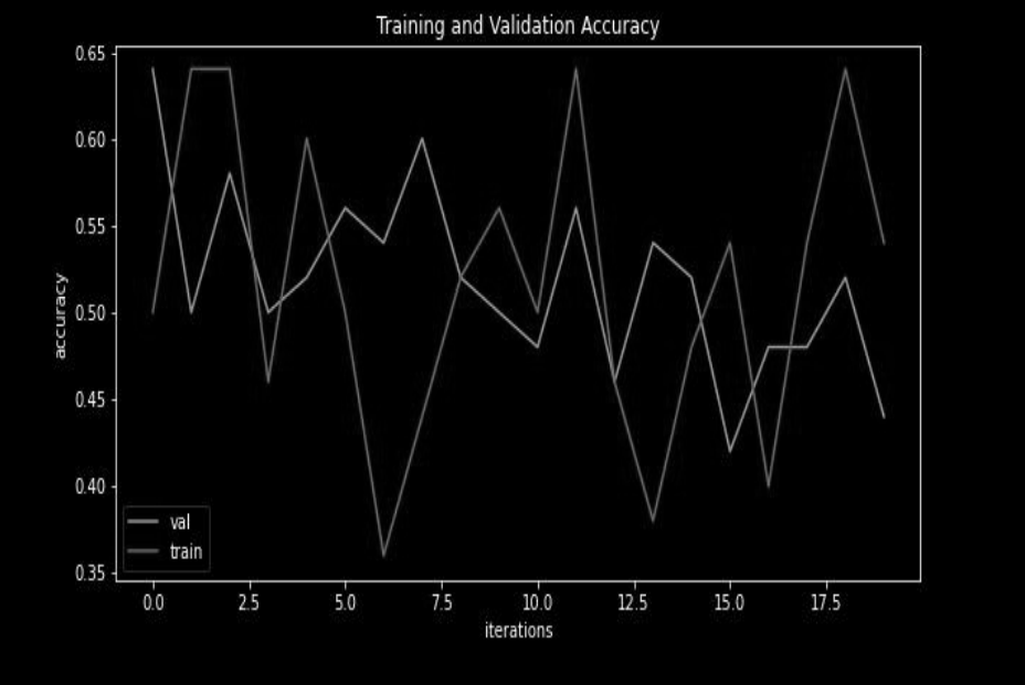
2. Mini-batch with SGD:
When the dataset is extensive, SGD can be utilized. Batch Gradient Descent quickly approaches minima. In the case of more enormous datasets, SGD converges more quicker. But we cannot use the vectorized implementation on SGD since we only use one sample at a time. The computations may get slower as a result.
Loss Curve:
In this curve, we have seen that both training and validation loss fluctuates as we increase the number of iterations or epochs.
Accuracy Curve:
In this curve, we have seen that both training and validation accuracy fluctuates as we increase the number of iterations or epochs.
3. Mini-batch SGD with momentum:
By accelerating gradient vectors in the proper directions, SGD with momentum is a strategy that promotes quicker convergence.
Loss Curve:
In this curve, we have seen that training and validation loss changes in the form of V shape mean decreases and then increases and remains constant as we increase the number of iterations or epochs.
Accuracy Curve:
In this curve, we have seen that both training and validation accuracy increases as we increase the number of iterations or epochs, which is expected using the basic concepts.
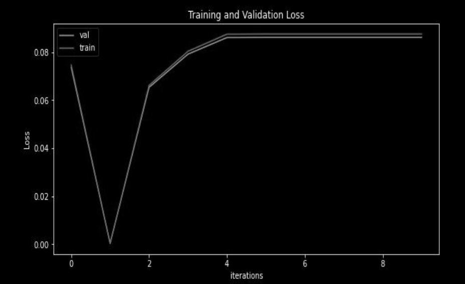
4. Mini batch with Adam:
Adam is an adaptive deep neural network training optimizer that has been successfully applied in many different fields. However, compared to stochastic gradient descent, its generalization performance on picture classification issues is much lower (SGD).
Loss curve:
In this curve, we have seen that both training and validation loss increases as we increase the number of iterations or epochs.
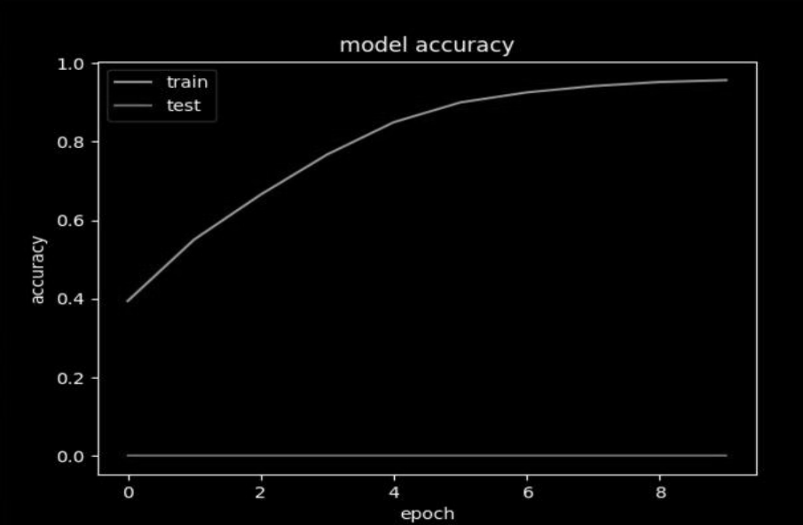
Accuracy Curve:
In this curve, we have seen that both training and validation accuracy remains constant as we increase the number of iterations or epochs.
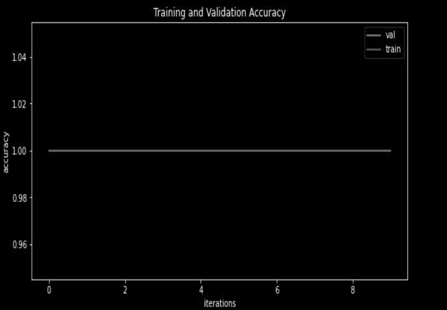
Image Classification Results
Initially, a mini-batch with SGD gives more accurate predictions on a small value of the number of epochs. Still, as we increase the number of epochs, after one point, we have observed that the mini-batch with momentum performs better as momentum also includes the previous variations in the current output. Hence, momentum optimization gives better accuracy over SGD.
For mini-batch with momentum, we use ADAM optimization, which uses the concept of both momentum and adaptive learning rate (which automatically sets the learning rate after each epoch based on the loss and accuracy we are getting). It means ADAM optimization will perform better for most of the problem statements.
Adam Optimizer will maintain two different hyperparameters – alpha and beta, which we can tweak and find the best possible accuracy since one factor is responsible for maintaining momentum and the other for learning rate adaptation.
Conclusion
You can download the complete code from this link.
So, finally, if we compare all four different models, we get the following order in terms of accuracy on the unseen dataset:
Mini batch with ADAM > Mini batch with SGD > Mini Batch with momentum > Vanilla SGD (This is not the hard and fast order, it varies with the dataset and problem statement, as we know that no universal classifier exists).
So, this concludes the given problem of image classification.
Significant takeaways from this article:
1. Firstly, we loaded and visualized the dataset. In this, we have read the images from the directory and then resized them into a fixed size. After that, split them into training and testing sets.
2. After that data pre-processing, we trained our CNN Model. While preparing our model, we applied several combinations of Conv2D layers, Max Pooling Layers, etc.
3. To further improve the accuracy, we have applied several optimization techniques like Vanilla SGD, Mini Batch SGD, etc.
3. Finally, we have concluded the article by discussing the best optimization technique, i.e., Mini batch with ADAM.
I hope you liked my article on image classification. Thanks for reading😊.
The media shown in this article is not owned by Analytics Vidhya and is used at the Author’s discretion.


