Introduction

Optimizing deep learning is a critical aspect of training efficient and accurate neural networks. Various  optimization algorithms have been developed to improve the convergence speed . One such Algorithm is Adahessian ,which is second-order optimization method known for its effectiveness in handling complex landscapes. In this article we will delve into the working of the ada hessian optimizer, compare it with first-order differential optimizer, and explore how it works and take steps to improve convergence.

For a comprehensive understanding, we will implement AdaHessian from scratch on a single neuron and visualize gradients in 3D plots. Our focus will be on analyzing the results of AdaHessian on this neuron and comparing it with Adam, visualizing the comparisons in 3D plots.

You can find the implementation details in the repository link.

Learning Objectives

• Gain insights into the differences between first-order and second-order optimization methods, their strengths, and limitations in training neural networks.
• Recognize the challenges faced by traditional optimization methods, such as computational cost, inaccurate Hessian approximation, and memory overhead.
• Learn about AdaHessian as a second-order optimization algorithm that addresses these challenges by incorporating Hessian diagonal approximation, spatial averaging, and Hessian momentum.
• Understand the fundamental components of AdaHessian, including the Hessian diagonal, spatial averaging for curvature smoothing, and momentum techniques for faster convergence.
• Explore the practical implementation of AdaHessian on a single neuron using NumPy, focusing on visualizing gradients in 3D plots and comparing its performance with AdamW.
• Develop a clear understanding of how AdaHessian leverages Hessian information, spatial averaging, and momentum to improve optimization stability and convergence speed.

 First-Order vs. Second-Order Optimization

• First-Order Optimization: First-order methods, such as Gradient Descent (GD) and its variants like Adam and RMSProp, rely on gradient information (first derivatives) to update model parameters. They are computationally less expensive but may suffer from slow convergence in highly non-linear and ill-conditioned optimization landscapes.

• Second-Order Optimization: Second-order methods, like AdaHessian, take into account not only the gradients but also the curvature of the loss function (second derivatives). This additional information can lead to faster convergence and better handling of complex optimization surfaces.

Lets understand about the  Second Derivative Curvature information :

Second-Order Derivatives

• The second derivative of a function  f(x)  at a point ( x ) gives us information about the curvature of the function’s graph at that point.
•  If the second derivative is positive at a point ( x ), it indicates that the function is concave up (bowl-shaped), suggesting a minimum point. This is because the function is curving upwards, like the bottom of a bowl.
•  If the second derivative is negative at a point ( x ), it indicates that the function is concave down (bowl-shaped), suggesting a maximum point. This is because the function is curving downwards, like the top of a bowl.
•  A second derivative of zero at a point ( x ) suggests a possible point of inflection. A point of inflection is where the curvature changes direction, such as transitioning from concave up to concave down or vice versa. However, further investigation is needed to confirm the presence of a point of inflection.

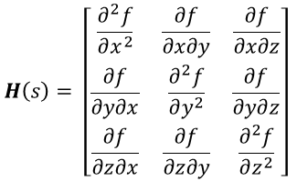
Hessian Matrix: For functions of multiple variables, the Hessian matrix is a square matrix that contains all the second-order partial derivatives of the function. The diagonal elements of the Hessian matrix correspond to the second partial derivatives with respect to individual variables, while the off-diagonal elements represent the mixed partial derivatives.

Curvature Information: The eigenvalues of the Hessian matrix provide crucial information about the curvature of the function at a given point.

1. If all eigenvalues are positive, the function is locally convex (bowl-shaped), indicating a minimum.
2.  If all eigenvalues are negative, the function is locally concave (upside-down bowl), indicating a maximum.
3. Mixed eigenvalues indicate saddle points or points of inflection.

So Now as we became familiar with some terms of second order optimization , lets deep dive into them 

Second Order Optimization 

Second-order optimization methods  handle bad conditioned optimization problems by considering both the direction and magnitude of curvature in the cost function. The Second order method can guarantees convergence while majority of first order method lack of  such guarantees.

Challenges Faced by Second-Order Methods

Second-order optimization methods, such as Newton’s method and Limited Memory BFGS (LBFGS), are commonly used due to their ability to handle curvature information and adjust learning rates automatically. 

However, they face challenges in machine learning tasks due to the stochastic nature of the problems and the difficulty in accurately approximating the Hessian matrix.

The main problems faced by second-order methods in machine are:

• Full Batch Gradients Requirement : Methods like LBFGS require full batch gradients, making them less suitable for stochastic optimization problems where using batch gradients can lead to significant errors in approximating the Hessian.
• Erroneous Approximation of the Hessian : Stochastic noise in the problem leads to inaccurate approximations of the Hessian, resulting in suboptimal descent directions and performance.
• Computational and Memory Overhead : The computational complexity of solving linear systems involving the Hessian, along with the quadratic memory complexity of forming and storing the Hessian, can be prohibitive for large-scale problems.

What is AdaHessian Algorithm?

To address these challenges, the AdaHessian algorithm proposes a solution that incorporates Hutchinson’s method along with spatial averaging. This approach reduces the impact of stochastic noise on the Hessian approximation, leading to improved performance in machine learning tasks compared to other second-order methods.

AdaHessian consists of three key components

• Hessian Diagonal Approximation 
• Spatial Averaging 
• Hessian Momentum 

Fundamental Concepts

Lets us consider that loss function is denoted by so as follow the notation corresponding gradient and hessian of f(w) at iteration t as gt and Ht .

Gradient Descent can be written as

Where 

• H : This represents a “Hessian” matrix in optimization 
• U: This represents a matrix containing the eigenvectors of H. The columns of U are the eigenvectors of H.
• Lambda: This is a diagonal matrix containing the eigenvalues of H. The diagonal elements of Lambda are the eigenvalues of H.
• U^T: This is the transpose of matrix U, where the rows of U^T become the columns of U and vice versa.

Hessian-Based Descent Directions

• A general descent direction can be written using the Hessian matrix and gradient as  where is the inverse Hessian matrix raised to a power k, and g_t is the gradient.
• The Hessian power parameter k controls the balance between gradient descent k=0 and Newton’s method k=1.

Note : in the context of the Hessian power parameter k, setting k=1 means fully utilizing Newton’s method, which provides accurate curvature information but at a higher computational cost. On the other hand, setting k=0 corresponds to simple gradient descent, which is computationally cheaper but may be less effective in capturing complex curvature information for optimization. Choosing an appropriate value of  k allows for a trade-off between computational efficiency and optimization effectiveness in Hessian-based methods.

Challenges with Hessian-Based Methods

• High Computational Cost : Naïve use of the Hessian inverse is computationally expensive, especially for large models.

•    Misleading Local Hessian Information : Local Hessian information can be misleading in noisy loss landscapes, leading to suboptimal descent directions and convergence.

Proposed Solutions

• Using Hessian Diagonal : Instead of the full Hessian, using the Hessian diagonal can reduce computational cost and mitigate misleading local curvature information.

• Randomized Numerical Linear Algebra : Techniques like Randomized Numerical Linear Algebra can approximate the Hessian matrix or its diagonal efficiently, addressing memory and computational complexity issues.

Hessian Diagonal Approximation

•  To address the computational challenge of applying the inverse Hessian in optimization methods, we can use an approximate Hessian operator, specifically the Hessian diagonal D.

• The Hessian diagonal is computed efficiently using the Hutchinson’s method, which involves two techniques: a Hessian-free method and a randomized numerical linear algebra (RandNLA) method.

•  The Hessian-free method allows us to compute the multiplication between the Hessian matrix H and a random vector z without explicitly forming the Hessian matrix.

• Using Hutchinson’s method, we compute the Hessian diagonal D as the expectation of  where z is a random vector with Rademacher distribution and Hz is computed using the Hessian matvec oracle.

• The Hessian diagonal approximation has the same convergence rate as using the full Hessian for simple convex functions, making it a computationally efficient alternative.
• Additionally, the Hessian diagonal can be used to compute its moving average, which helps in smoothing out noisy local curvature information and obtaining estimates that use global Hessian information.

This process allows us to efficiently approximate the Hessian diagonal without incurring the computational cost of forming and inverting the full Hessian matrix, making it suitable for large-scale optimization tasks.

Spatial Averaging for Hessian Diagonal Smoothing

AdaHessian employs spatial averaging to address the spatial variability of the Hessian diagonal, particularly beneficial for convolutional layers where each parameter can have a distinct Hessian diagonal. This averaging helps in smoothing out spatial variations and improving optimization stability.

Mathematical Equation for Spatial Averaging

The spatial averaging of the Hessian diagonal can be expressed mathematically as follows:

Where:

• D(s) is the spatially averaged Hessian diagonal.
• D  is the original Hessian diagonal.
• P  is the spatial average block size.
• i  and  j are indices referring to elements of D and  D(s) , respectively.
• b  is the spatial average block size.
• d is the number of model parameters divisible by b.

Spatial Averaging Operation

•  We divide the model parameters into blocks of size b and compute the average Hessian diagonal for each block.
•  Each element in the spatially averaged Hessian diagonal D(s)  is calculated as the average of corresponding elements in D within the block.

Benefits of Spatial Averaging

• Smoothing Out Variations: Helps in smoothing out spatial variations in the Hessian diagonal, especially beneficial for convolutional layers with diverse parameter gradients.
• Optimization Stability: Improves optimization stability by providing a more consistent and reliable estimate of the Hessian diagonal across parameter dimensions.

This approach enhances AdaHessian’s effectiveness in dealing with spatially variant Hessian diagonals, contributing to smoother optimization and improved convergence rates, particularly in convolutional layers.

What is Hessian Momentum?

AdaHessian introduces momentum techniques to the Hessian diagonal, enhancing optimization stability and convergence speed. The momentum term is added to the Hessian diagonal, leveraging its vector nature instead of dealing with a large matrix.

Mathematical Equation for Hessian Diagonal with Momentum

The Hessian diagonal with momentum D_t is calculated using the following equation:

Where:

• D(s) is the spatially averaged Hessian diagonal.
• beta_2  is the second moment hyperparameter (0 < beta_2 < 1 ).
• s  is a scaling factor.

AdaHessian Algorithm Steps

Let us now have a look at all the AdaHessian Algorithm steps:

Step1: Compute Gradient and Hessian Diagonal

• g_t  ← current step gradient
• D_t  ← current step estimated diagonal Hessian

Step2: Compute Spatially Averaged Hessian Diagonal

• Compute using below equation 

Step3: Update Hessian Diagonal with Momentum

• Update  Dt using this equation

Step4: Update Momentum Terms

• Update m_t and v_t  

Step5: Update Parameters

AdaHessian Algorithm (Pseudocode)

Requirements for the AdaHessian Algorithm are:

• Initial Parameter: θ0
• Learning rate: η
• Exponential decay rates: β1, β2
• Block size: b
• Hessian Power: k
• Set: m0 = 0, v0 = 0
• for t = 1, 2, . . . do // Training Iterations
  • gt ← current step gradient
  • Dt ← current step estimated diagonal Hessian
  • Compute D(s)t 
  • Update Dt 
  • Update mt, vt
  • θt = θt−1 – η * mt/vt

Hessian Diagonal with Momentum : D_t  incorporates momentum to the Hessian diagonal, aiding in faster convergence and escaping local minima.

Algorithm Overview : AdaHessian integrates Hessian momentum within the optimization loop, updating parameters based on gradient, Hessian diagonal, and momentum terms.

By incorporating momentum to the Hessian diagonal, AdaHessian achieves improved optimization performance, as demonstrated in the example showcasing faster convergence and avoiding local minima.

Now that we’ve thoroughly grasped the theory behind AdaHessian, let’s transition to putting it into practice. 

Implementation and Result Analysis

We’ve implemented AdaHessian to train a single sigmoid neuron with one weight and one bias using one input. The configuration and data remain consistent throughout the experiments.

After training, we analyzed the loss and parameter change graphs. You can find the implementation code in the GitHub repository.

We won’t be testing this model as it’s specifically designed for analyzing AdaHessian and its superiority over first-degree algorithms.

This analysis aims to evaluate AdaHessian’s efficiency in optimizing the neuron and to gain insights into its convergence behavior. Let’s delve into the detailed analysis and visualizations.

Loss Analysis

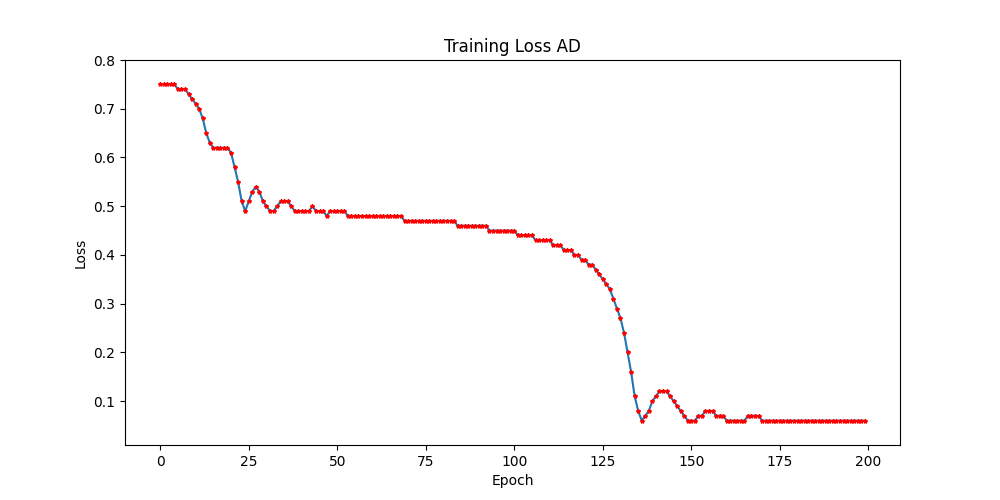
The training loss graph shows how the model’s error decreases over 200 epochs with AdaHessian optimization.
Initially rapid, the loss reduction slows later, suggesting convergence. Fluctuations around epochs 100-150 indicate possible noise or learning rate adjustments. AdaHessian effectively optimizes the model by adjusting learning steps using second-order derivative information.

Now Let’s visualize error or loss function of our sigmoid neuron in Using 2D and 3D Graphs .

2D Graphs

Here we are plotting the loss surface of the Neuron in 2d:

• The contour lines represent levels of the loss function value. The red areas correspond to higher loss values, and the blue areas correspond to lower loss values. Ideally, the optimization algorithm should move towards the blue areas where the loss is lower.
• The black dot represents the current values of weight (w) and bias (b) at this epoch. Its position on the plot suggests the initial parameters before training starts.
• As each epoch progresses with the AdaHessian optimizer updating weights and biases, the gradient steadily descends towards the minima. The changing values of weights create a trajectory of optimization, gradually moving towards the minima, resulting in a decrease in error as well.

3D Graphs

Lets visualize the Loss function of the neuron in 3D  for better visualization.

It provides a visual representation of the loss surface with respect to the weight (w) and bias (b) of a single neuron model, with the third axis representing the loss value.

• Axes : The horizontal plane represents the parameters—weight (w) on one axis and bias (b) on another. The vertical axis represents the loss value.
• Contourplot and Surface  : Underneath the surface, the contour plot is visible. It represents the same information as the surface but from a top-down view. The contour lines help to visualize the gradient (or slope) of the surface
• Optimization Path : The black line shows how our optimization process moves towards the lowest point in the 3D plots. In the 2D figure or surface of this , you can see this as the red line tracing the same path downward towards the minimum.

So the visualizations depict the loss surface of a sigmoid neuron using 2D and 3D plots. Contour lines in 2D show different loss levels, with red for higher and blue for lower losses.

The black dot represents initial parameters, and the optimization path demonstrates descent towards lower loss values. The 3D plot adds depth, illustrating the loss surface with weight, bias, and loss value. 

Now After Analyzing results let’s compare it with Adam with same set of configuration but these result are extracted using the pytorch frame work for more information about the implementation follow github link here.

Loss of Adam and AdaHessian in Training Phase

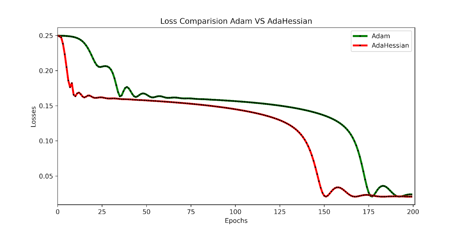
The AdaHessian loss stabilizes after 150 epochs, indicating that the optimization process reaches a steady state. On the other hand, the Adam loss continues to decrease until it also stabilizes at 175 epochs, aligning with the AdaHessian loss trend. This shows that AdaHessian effectively optimizes the model by leveraging second-order derivative information, which allows for precise adjustments in learning steps to achieve optimal performance.

Lets Visualize this Comparison in the 2d and 3d for the better understanding of the optimization process.

Visual Comparison in 2D Graphs 

In this  2D contour plot comparing the loss surface traversal of two different optimization algorithms: Adam and AdaHessian. The axes w and b represent the weight and bias parameters of a neuron, while the contour lines indicate levels of loss.

• Path Comparison : There are two paths marked on the plot, one for Adam (black) and one for AdaHessian (red). These paths show the trajectory of the weight and bias values as they are updated by their respective algorithms during training.
• Starting Points : Both paths start at the same point, indicated by the intersection of the two dotted lines, suggesting that both algorithms began with identical initial conditions for weight and bias.
• Algorithm Performance : Although it’s just the initial point, the fact that both errors are equal suggests that at this very early stage in training, both optimizers are performing equivalently.
• Trajectories and Learning Dynamics : The paths show the direction each optimizer is taking to minimize the loss.As we can see Over subsequent epochs, these paths illustrate how each optimizer navigates the loss surface differently, potentially converging to different local minima or the global minimum.
• Contour Gradients : The gradients of the contour lines give us an indication of how the loss changes with respect to w and b. Steeper gradients mean more significant changes in loss with small changes in parameters, while flatter areas indicate less sensitivity to parameter changes.
• Results : As we can see that red line(adahessian) moving to the minima faster or in less epochs than the blackline(Adam).So Adahessian converging faster than the Adam Though

To make this comparison more understandable Lets analyse this comparison in 3D Plot.

Visual Comparison in 3D Graphs :

Contours in 3D plots provide a comprehensive view of the function’s variations. In this analysis, we focus on the trajectory comparison between AdaHessian and Adam in a 3D plot.

• Trajectory Comparison: The 3D plot displays the trajectory of optimization for AdaHessian (red) and Adam (green). AdaHessian’s trajectory shows a more direct path towards the minima compared to Adam.
• Optimization Dynamics: The contours in the 3D plot illustrate how the loss function changes with different weight and bias combinations. Steeper contours indicate areas of rapid loss change, while flatter contours represent slower changes.
• Results Interpretation: From the 3D plot, it’s evident that AdaHessian converges faster and follows a more efficient path towards the minimum loss compared to Adam.

This analysis in the 3D plot provides a clear visual understanding of how AdaHessian outperforms Adam in terms of optimization speed and efficiency.

Conclusion

AdaHessian shows great promise in addressing challenges faced by traditional optimization methods in deep learning. By leveraging second-order information, spatial averaging, and momentum techniques, AdaHessian boosts optimization stability, speeds up convergence, and navigates complex landscapes more effectively.

The analysis of our plots revealed that AdaHessian’s loss stabilizes after 150 epochs. This indicates steady optimization, whereas AdamW continues to decrease until stabilizing at 175 epochs. Visualizing the trajectories in 2D and 3D plots clearly demonstrated that AdaHessian converges faster and takes a more efficient path towards minimum loss compared to AdamW.

This theoretical and practical comparison underscores AdaHessian’s superiority in optimizing neural networks, especially in terms of convergence speed and efficiency. As deep learning models advance, algorithms like AdaHessian contribute significantly to improving training dynamics, model accuracy, and overall performance. Embracing advancements in optimization techniques opens doors to substantial progress in deep learning research and applications.

Key Takeaways

• AdaHessian is a second-order optimization algorithm designed to address challenges in traditional optimization methods for deep learning.
• Second-order methods face issues like requiring full batch gradients, inaccurate Hessian approximations, and high computational and memory overhead.
• The AdaHessian algorithm involves computing gradients, Hessian diagonals, spatially averaged diagonals, updating momentum terms, and updating parameters for efficient optimization.
• Visualizing AdaHessian and Adam in 2D and 3D plots demonstrates AdaHessian’s faster convergence and more efficient trajectory towards minimum loss.

Frequently Asked Questions