From Word Embedding to Documents Embedding without any Training

This article was published as a part of the Data Science Blogathon. 

Introduction

Pre-requisite: Basic understanding of Python, machine learning, scikit learn python, Classification

Objectives: In this tutorial, we will build a method for embedding text documents, called Bag of concepts, and then we will use the resulting representations (embedding) to classify these documents. First, I’ll briefly explain what the BOC is and then start implementation using Python

Implementation phases:

1. Preprocessing BBC data set.
2. Training the FASTEXT word embeddings model on BBC data set.
3. Formation of the so-called dictionary of words embeddings.
4. Clustering words: Apply a clustering algorithm to embedded words to form concepts.
5. Concepts extraction: Use concepts to encode documents and generate concept vectors according to CF-IDF format.
6. Training an SVM classifier to classify documents using generated vectors.
7. Performance evaluation using F-score and confusion matrix.

 

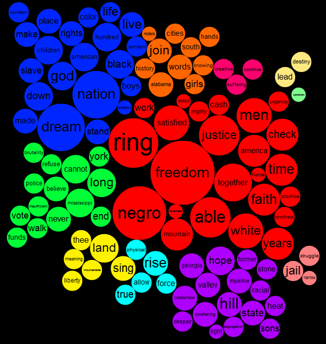
Clusters of words. Source: https://neoformix.com/2011/WordClusterDiagram.html

What is Bag-of-concepts

The BOC (Bag-of-Concepts) method has been proposed as a solution to the problem of large dimensions that traditional methods such as TF-IDF and Bag of words suffer from. Based on the corpus of a collection of documents, BOC encodes words as embedding vectors and then applies clustering to group similar words into clusters called concepts. As with the BOW method, each document vector will be represented by the frequencies of these concepts in the document. A weighting scheme similar to TF_IDF is used, replacing the term TF frequency with the CF concept frequency. Hence, it is called CF-IDF (Concept Frequency with Inverse Document Frequency) and is calculated based on the following equation.

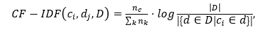
where |D| – the number of documents in the collection, and the denominator is the number of documents from the collection D, in which the concept c occurs; n_c is the number of occurrences of concept c in document d, and n_k is the total number of concepts in this document.

BBC Dataset preprocessing

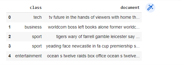
BBC dataset, consists of 2225 documents from the BBC news website covering stories in five topical areas from 2004-2005. It includes five categories: tech, business, sport, entertainment, and politics. We assume that our data is stored on the drive within the specified path. The sample consists of the document text and the category. The data file is CSV type, so we use read_csv function. Then I change the column names (this is optional).

import pandas as pd
BBC_file_path="/content/drive/...../Data/bbc-text.csv"
data_DF = pd.read_csv(BBC_file_path)
# rename columns
data_DF.columns.values[0] = "class"
data_DF.columns.values[1] = "document"
data_DF.head()

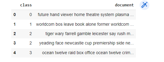
As you can see classes are labels that must be converted into numbers so that they can be dealt with by the classifier later. For this, we use the factorize function:

# Factorize class names to numbers
data_DF['class'] = pd.factorize(data_DF['class'])[0]

Then we do the pre-processing of the documents to remove the noise. Processing includes lemmatization, tokenization, and removing (stop words, whitespace, punctuation marks, numbers, etc). This is not the focus of the article so we’ll let the code speak for itself.

data_DF['document'] = data_DF.document.apply(lambda x: ' '.join(preprocess_text(x)))
data_DF.head()

Here are the text processing functions

import re
import string
import numpy as np
import math
from numpy import array 
import nltk
from nltk.tokenize import word_tokenize
from nltk.corpus import stopwords 
from sklearn.cluster import KMeans
from collections import Counter 
nltk.download('averaged_perceptron_tagger')
nltk.download('punkt')
nltk.download('stopwords')
nltk.download('wordnet')
#-------------------------------------------------------------------------------
from nltk.stem import WordNetLemmatizer
from nltk import word_tokenize, pos_tag
#-------------------------------------------------------------------------------
def preprocess_text(text):
    text = re.sub(r'd+' , '', text)
    text = remove_punctuation(text)
    text = text.lower()
    text = text.strip()
    text = re.sub(r'bw{1,2}b', '', text)
    tokens = toknizing(text)
    pos_map = {'J': 'a', 'N': 'n', 'R': 'r', 'V': 'v'}
    pos_tags = pos_tag(tokens)
    lemmatiser = WordNetLemmatizer()
    tokens = [lemmatiser.lemmatize(t.lower(), pos=pos_map.get(p[0], 'v')) for t, p in pos_tags]
    return tokens

#--------------------------------------------------------------------------------------------
def remove_punctuation(text):
     punctuations = '''!()-[]{};:'",./?@#$%^+&*_~'''
     no_punct = ""
     for char in text:
        if char not in punctuations:
            no_punct = no_punct + char
     return no_punct
#--------------------------------------------------------------------------------------------
def toknizing(text):
  stop_words = set(stopwords.words('english'))
  tokens = word_tokenize(text)
  result = [i for i in tokens if not i in stop_words]
  return result

Training the FASTEXT word embeddings model on BBC data set

Next, we import the gensim library and choose the Fasttext model. Fastext takes several parameters, the most important of which are:

# Train fast text model on your dataset
import gensim
from gensim.models import FastText
documents_as_list = data_DF['document'].tolist()
doc_as_tokens =[]
for doc in documents_as_list:
  doc_as_tokens.append(doc.split())

model = FastText(doc_as_tokens, size=300, window=15, min_count=5, workers=4,sg=1)

Therefore, the document series must be converted into a list of documents consisting of a list of tokens (doc_as_tokens). We set the parameters as shown in the code. Then execute it!!

After training the model on the BBC data, we can extract the words and their vectors. We are going to build a dictionary dic_w_v in which the key is the word as text, and the value is its corresponding vector. Also, we will represent each document as a list of embedded words and store them in all_doc_emb. Through the following code:

dic_w_v = {}
all_doc_emb = []
for doc in doc_as_tokens:
  doc_emb = []
  for w in doc:
    try :
      emb = model.wv[w]
      doc_emb.append(emb)
      dic_w_v.update({w : emb})
    except: 
      continue;
  all_doc_emb.append(doc_emb)

Clustering the words embeddings

The next step is the formation of the so-called dictionary of words embeddings. So we want to group similar words together into clusters called concepts. We use a spherical k-means algorithm which adopts cosine similarity as a criterion for similarity.

!pip install soyclustering
from soyclustering import SphericalKMeans
from scipy.sparse import csr_matrix
#-------------------------------------------------------------------------------
def spherical_kmeans(n_clusters_, list_of_words_vectors,sim_digree):
  embeddings_matrix_csr = csr_matrix(list_of_words_vectors)
  spherical_kmeans = SphericalKMeans( max_similar=sim_digree, init='similar_cut', 
      n_clusters = n_clusters_)
  labels = spherical_kmeans.fit_predict(embeddings_matrix_csr)
  centers = spherical_kmeans.cluster_centers_
  return labels , centers

You must first install soyclustering and then import SphericalKMeans. We also need to convert the embedding arrays to csr so the SphericalKMeans function can handle it.

The function takes the following parameters: a number of clusters, similarity threshold, and a list of embedding vectors, and returns cluster centers and labels. Note that the centers of the clusters are embedding vectors with the same dimension as the word vectors 300. From the dictionary, we just take the vectors of words and store them as a list. We set the parameters as in the code.

list_of_words_vectors = list(dic_w_v.values())
# number of clusters
K_clusters= 200
sim_digree=0.3
######### Clustering
labels , centers = spherical_kmeans(K_clusters , list_of_words_vectors, sim_digree)

Clusters represent concepts. The centroid vector is a representative of the concept that groups the words of the cluster around it.

Concepts extraction

Now we have the clusters (concepts) and we have each document represented by its own embedded words. We want to construct a vector representation of the document so that each element in it expresses the degree to which the concept is present in the document (the weight of the concept). This weight is calculated according to the formula CFIDF.

For this I built a BOC function that creates for each document one vector, each element being the frequency of a concept in the document. The function accepts the following parameters: the document as a list of its words’ vectors, the similarity threshold, and the clusters’ centroids vectors. This function BOC is called within the second function CF_IDF_BOC. So we will explain how BOC works first and then move to the parent function.

final_embeddings  = CF_IDF_BOC(all_doc_emb , alpha , centers)

Within the BOC function, an empty matrix is created to store the frequencies of concepts, the number of its elements equals the number of concepts. Next we have a loop that goes through the centers of the clusters. The similarity of each word of the document is compared with all centers. If the degree of similarity is greater than the specified threshold, the concept counter is increased by one, otherwise, it does not change. In this way, we calculate the occurrences of each concept in the document, then we can calculate the frequency as the occurrence of the concept divided by the sum of the occurrences of all concepts. These values are then stored in the conceptual frequency matrix.

#Get concepts frequencies vector for a single document
def BOC(embeddeings_document,alpha,centers):
  concept_occurence = 0
  ## intilize doc array
  CF_vector = np.zeros(len(centers)).tolist()
  for cnt in range(len(centers)):
    for emb_word in embeddeings_document:
      Wsim= cosine_distance(emb_word , centers[cnt])
      if Wsim  > alpha:
        concept_occurence = concept_occurence + 1 #for tf
        CF_vector[cnt] = CF_vector[cnt] + 1;
      else:
        continue;    
  if concept_occurence !=0:
    for i in CF_vector:
      i = i / concept_occurence  #count/
  return CF_vector

The CF_IDF_BOC function is the parent function that for each document calls the BOC function that returns a concept vector containing the frequencies of the concepts and then calculates the inverse frequency of the documents based on the BOC output, then multiplying the concept frequency by the inverse frequency of the document to produce the final weight CF-IDF

def CF_IDF_BOC(documents_embeddings , alpha , centers):
  CFs = []
  counter = 0
  Df = np.zeros(len(centers)).tolist() # equal to the clusters count
  for doc in documents_embeddings: 
    CF = BOC(doc , alpha , centers )
    for i in CF: 
      if i > 0:
        Df[counter] = Df[counter] + 1 #  i[M-1]
      counter = counter+1
    counter = 0
    CFs.append(CF)
  #########  calculate IDF
  IDF=[]
  for df in Df:
    if df!=0:
      N=len(documents_embeddings)
      IDF.append( math.log10( (N+1) /df ) )
    else:
      IDF.append(0)  
  #Calculate Cf-IDF
  for i in range(N):
    l=len(CFs[i])
    for j in range(l):
       CFs[i][j] = CFs[i][j] * IDF[j]  #cf*idf
  return CFs

The time to build document vectors varies depending on the number of concepts, and the number of documents in the data set.

Training an SVM classifier

We have got embedding vectors for documents with dimensions of 200 features. Now we will convert the labels to a list. Then we split the data: 30% for testing and the rest for training. We pass the resulting vectors, class labels and the sample size to the train_test_split function:

from sklearn.model_selection import train_test_split
from sklearn.svm import SVC
from sklearn.metrics import f1_score
#-------------------------------------------------------------------------------
classes = data_DF['class'].tolist()
x_train , x_test , y_train , y_test = train_test_split(final_embeddings , classes , test_size = 0.30 , random_state = 0)

After that we can build and train an SVM classifier using training samples. All types of kernels can be tested. Here we found that the RBF is the best

svm =  SVC(kernel='linear', random_state=44).fit(x_train , y_train)

Performance evaluation using

To evaluate the performance of the SVM classifier we will use the accuracy and macro-average f1 score as you can see. For that let us import the classification_report:

from sklearn.metrics import classification_report
y_pred=svm.predict(x_test)

print(classification_report(y_test, y_pred))

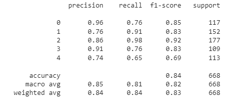
The accuracy according to the F1 score is 84%, which is very good, considering the low number of features. Accuracy can vary, increase or decrease since it depends on the results of the unsupervised word-clustering algorithm.

Recommendations to improve performance: The number of words used to build the concept dictionary can be reduced by keeping only words that appear more than a certain limit (20 times). This allows only the important words to participate in building the concept dictionary.

Conclusion

In this tutorial, we have presented an implementation of a method for generating embeddings for documents based on the embeddings of individual words. The next step will be to compare the performance of this method with others that are strong baselines in text classification tasks (Doc2vec, TF-IDF,….) using different standard data sets. You can check the code on my repository at GitHub. I would be grateful for any feedback.

What else? If you need to know how to extract keyphrases from documents using the TF-IDF method please  Click here

About me: My name is Ali Mahmoud Mansour, currently (in 2022) I am a graduate student (Ph.D. researcher) in the field of computer science. Passionate about text mining and data science.

References

Mansour, Ali Mahmoud, Juman Hussain Mohammad, and Yu. A. Kravchenko. “VECTORIZATION OF TEXT USING DATA MINING METHODS.” Izvestia SFedU. Technical science. 2 (2021).

Kim, H. K., H.-j. Kim and Cho (2017). “Bag-of-concepts: Comprehending document representation through clustering words in distributed representation.” Neurocomputing 266: 336-352.

BBC dataset you can download here

Ali Mansour 05 Jan 2022