Introduction to Graph Data Science

This article was published as a part of the Data Science Blogathon.

Introduction

In this blog post, I will summarise graph data science and how simple python commands can get a lot of interesting and excellent insights and statistics.

It has become one of the hottest areas to research in data science and machine learning in recent years due to the comprehensive research and application of graph-based machine learning techniques in fields like social networking, molecular relationship analysis, recommendation systems in eCommerce stores, etc.

To begin with, I will explain the most popular terminology and concepts from graph theory, a branch of mathematics. Then we will look at how the graph data is structured and the various actions that can be performed by walking you through the code examples side by side. I will be using the networkx python library here to illustrate this. I will discuss state-of-the-art topics like graph convolutional networks with code examples in the succeeding posts.

Graph Theory Basics

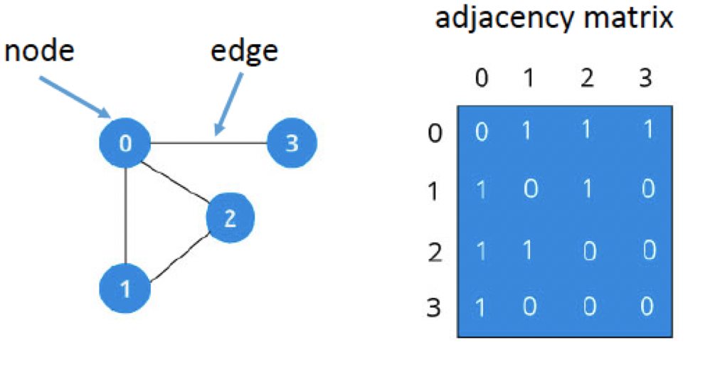
A graph is an ordered pair of G (V, E), where V is the set of Vertices or Nodes and E is the set of Edges or relationships connecting those Nodes such that E ⊆ {(x, y) | x, y ∈ V, and x ≠ y. Refer fig below

Source: https://andysbrainbook.readthedocs.io/en/latest/FunctionalConnectivity/CONN_ShortCourse/CONN_AppendixA_GraphTheory.html

Any G is a 2-dimensional array with rows and columns representing the Nodes in the graph.

Adjacency Matrix:

An adjacency matrix is a square Boolean matrix (comprising of 0’s and 1’s only) representing the graph where the rows and columns are the Nodes of the graph. The M(I, J) value of 1 indicates that Nodes I and j have a direct connection or relationship, and the M(I, J) value of 0 indicates that Nodes I and j do not have a direct relationship with each other.

Types of Graphs: 

Graphs can be directed or undirected graphs

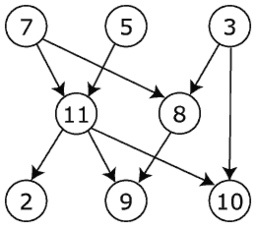
Directed and undirected Graph:

In the directed graph, the nodes and links are connected where all the edges are directed from one vertex to another, whereas an undirected graph is a set of nodes and links between the nodes.

Source File: Directed graph, cyclic.svg – Wikimedia Commons

Source Graph theory – Wikipedia

Cyclic Graph and loops:

Loops: 

In graph theory, a loop or a self-loop is a node that connects a vertex to itself.

Cyclic and Acyclic graphs: 

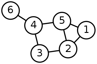
Whenever in a graph, a few vertices are attached in a closed chain of relations, then the graph is said to have a cycle. A graph with at least one such cycle is called the cyclic graph, and the graph with zero cycles is an acyclic graph. In the above-undirected graph, the nodes 2,3,4,5 form a cycle

With this knowledge, let’s go to Jupiter lab (or colab or python editor of your choice) and create our first Graph

First, we need to install the python graph library. In this post, I am using Networkx and colab environment. There are other graph database tools like Neo4j to work with graphs.

!pip3 install networkx

Now import a few libraries to work with Graphs

import networkx as nx
print(nx.__version__)

Create an empty undirected Graph

G = nx.Graph()  # for directed graph use this command G = nx.DiGraph()

Now, graph G does not have any Nodes or Links yet. Let us create them as in the figure above

Nodes = list(range(1,7))
G.add_nodes_from(Nodes)   # Creates nodes from 1,2,.. 6

Now let us add a few links to the graph.

To view the graph, write the below code and run it

nx.draw(G)

The main purpose of networkx is to assist in graph analysis and not graph visualization. For graph visualization, we can use other tools like Gephi, Graphviz, etc. for more details; you can refer to the networkx documentation page link – Drawing — NetworkX 2.8.5 documentation – Drawing — NetworkX 2.8.5 documentation

The Graph Data Structure

As we have seen, graph G must have a set of nodes and a relationship with some other nodes to form a link connection. Every node in a graph can have attributes associated with it. For example, if different locations in a city form nodes of a certain graph, then pin code, latitude, longitude, etc., can be its attributes. Similarly, every link in a graph can have unique attributes; for example, we can add a ‘weight’ to each link to represent the distance between the two connecting locations or nodes. Also, in our real-time data, it will not be easy to add all the nodes, their links, and their attributes. There is an easy way to do this in python using dictionaries which I will show below. For this article, which is primarily to introduce graph data science concepts, we will create the data ourselves and then perform some operations. This should give you a good idea to go about when working with a Real-time dataset

First, we will create 100 random nodes, and each node will have at most 2 links and assign random weights to each of the links in the graph. We will exclude self-loops for now and the undirected graph. Code for this below

from random import random
import random
import numpy as np
import matplotlib.pyplot as plt

nodes = list(range(1,100))
G = nx.Graph()   # create undirected graph
for n in nodes: # traverse through the nodes list above which has 100 numbers
  for i in range(0,2):
    n1 = random.randint(1,100)
    if n==n1 :   # ignore self loops
      continue
    w1 = np.round(random.random(),2)
    G.add_edge(n,n1,weight=w1)  # add random weights to edges 
len(G.nodes),len(G.edges)

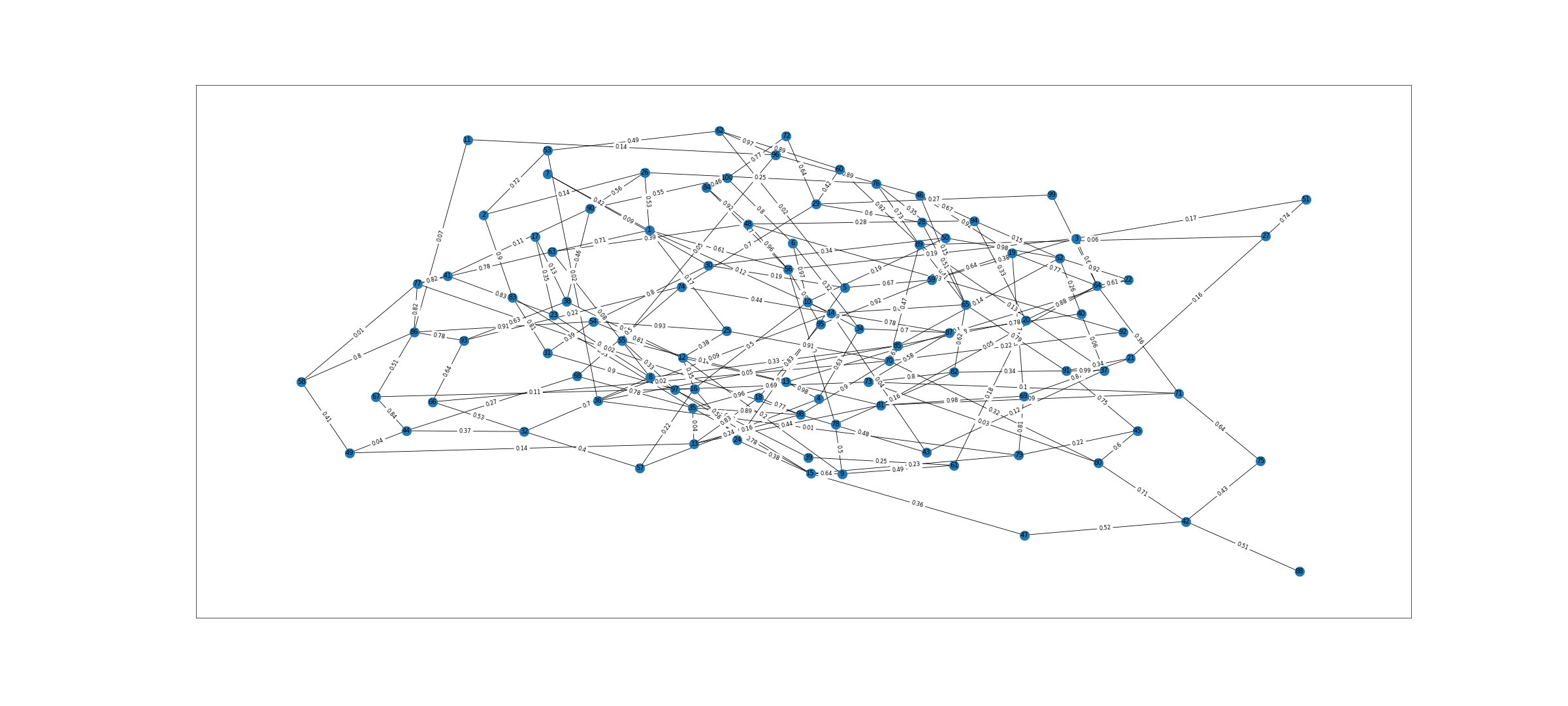
We can now see 100 nodes and 191 edges created in this graph. We can visualize it as below

fig = plt.figure(1, figsize=(40, 18), dpi=60)
pos=nx.spring_layout(G) # pos = nx.nx_agraph.graphviz_layout(G)
nx.draw_networkx(G,pos)
labels = nx.get_edge_attributes(G,'weight')
nx.draw_networkx_edge_labels(G,pos,edge_labels=labels)
#nx.draw(G,with_labels=True,font_weight='normal')
plt.show()

Graph

Graph Operations

Before performing some operations on the graph, we created above, let us look at a few more concepts from graph theory that are used in graph data science

Path in Graph: 

A path in a graph is a finite or infinite sequence of edges connecting distinct vertices between two nodes. In a directed graph, the node order cannot be reversed.

Shortest Path between any two nodes in a graph: 

The path between two nodes that has the least sum of the weights of its constituent links is the shortest path. For example, in below figure shortest path (A, C, E, D, F) between vertices A and F in the weighted directed graph is 2+3+4+11 = 30

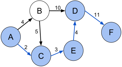
Source: Shortest path with direct weights – Shortest path problem – Wikipedia

Length of a Graph: 

It is the total number of links in the graph

The eccentricity of a Graph: 

It is the maximum distance of one vertex from another vertex. The eccentricity of a vertex is the maximum distance between the vertex to all the other vertices.

Radius and Diameter of a Graph: 

It is the minimum and maximum eccentricity in the graph. If the graph diameter is ‘N’, then it has N hop neighbors in it. This is a key metric for deciding the number of layers in the GNN – Graph Neural Networks.

The density of a Graph: 

The density of the graph is calculated using the below formula

For undirected graph – d = 2m /n * (n-1)

For a directed graph, it is m/n *(n-1)

Where n is the number of nodes and m is the number of links in the graph.
A graph that has no links will have 0 density, and a graph where all pairs of distinct nodes will have a link connecting them will have a density on 1 unit

PageRank of a Graph: 

This is another key metric while working with graph data. It ranks the nodes according to their importance in the graph. If the input graph is undirected, this will be converted to a directed graph with two directed links for each undirected link. Since we are working on the randomly created graph, there will be skewness, but when we are working with the real dataset, this will give beneficial insights and can be used for node feature embedding, a concept used in GCN – Graph Convolutional Networks

Node Degree: 

In an undirected graph, it is the sum of all linked nodes to it, and in a directed graph, the in-degree is the number of nodes leading into it, and the out-degree is the number of nodes leading out from that node.

Let us check the above for the graph we created

import operator

Length = len(G.edges)   # length of the Graph – 193
eccentricity =  nx.eccentricity(G) # nx.eccentricity(G)[10] to check eccentricity for node 10
radius = nx.radius(G)   # 4
diameter = nx.diameter(G) # 7
density = nx.density(G)  # 0.038585858585858585
shortest_path_1_100 = nx.shortest_path(G,1,100) # [1, 33, 98, 88, 100])
pr = nx.pagerank(G,alpha=0.9)
print(sorted(pr.items(), key=operator.itemgetter(1), reverse=True)[0:5])
# Top five nodes of importance based on page rank -- [(7, 0.023270691594625876), (23, 0.020206209312297146), (63, 0.019264125648625598), (24, 0.018898324997949915), (4, 0.01869535054804308)] 
ndeg = G.degree(nodes)  # Node degrees will be printed like 
Print(ndeg)

DegreeView({1: 3, 2: 5, 3: 4, 4: 3, 5: 2, 6: 6, 7: 2, 8: 3, 9: 3, 10: 5, 11: 3, 12: 5, 13: 3, 14: 3, 15: 4, 16: 3, 17: 4, 18: 4, 19: 4, 20: 4, 21: 4, 22: 3, 23: 2, 24: 3, 25: 4, 26: 9, 27: 6, 28: 4, 29: 5, 30: 4, 31: 3, 32: 3, 33: 6, 34: 2, 35: 4, 36: 3, 37: 3, 38: 8, 39: 5, 40: 2, 41: 3, 42: 3, 43: 5, 44: 3, 45: 5, 46: 7, 47: 5, 48: 4, 49: 3, 50: 3, 51: 5, 52: 3, 53: 3, 54: 3, 55: 4, 56: 5, 57: 3, 58: 3, 59: 3, 60: 5, 61: 2, 62: 4, 63: 2, 64: 4, 65: 4, 66: 2, 67: 2, 68: 4, 69: 6, 70: 2, 71: 6, 72: 5, 73: 1, 74: 5, 75: 4, 76: 2, 77: 1, 78: 7, 79: 3, 80: 4, 81: 2, 82: 4, 83: 4, 84: 5, 85: 6, 86: 3, 87: 2, 88: 4, 89: 4, 90: 3, 91: 5, 92: 5, 93: 3, 94: 4, 95: 3, 96: 5, 97: 4, 98: 4, 99: 4})

Now that we have 2 metrics at node level viz – PageRank and node degree, let us set these as node attributes in our graph.

node_page_rank = {}
node_degree    = {}
for node in nodes:  # traverse through the nodes
  node_page_rank[node] = pr[node]
  node_degree[node] = ndeg[node]
nx.set_node_attributes(G, node_page_rank, 'PageRank')  # set attribute
nx.set_node_attributes(G, node_degree, 'nodeDegree')  # set attribute
for n in nodes: # Loop through every node
    print(n, G.nodes[n]['PageRank']) # Access every node by its Rank"

Also, we can access the nodes by their degree. Likewise, we can also set link attributes based on our use cases.

Node Neighbors in Graph: 

Node v is the neighbor of Node u if a connection exists between
(u,v). In the figure above, the neighbors of node 5 are nodes 1,2,4. Often during our analysis, we may require information about the neighbors of a node. In the below code, we get all the neighbors of any node in the graph and find the weights of the edges and attributes of the connecting nodes.

from networkx.classes.function import all_neighbors
u =50
v =[n for n in all_neighbors(G,u)]
for v in v:
  print(u,v,G.get_edge_data(u,v),"Degree ",G.nodes[v]['nodeDegree'],"Rank ",G.nodes[v]['PageRank'])

50 38 {'weight': 0.65} Degree  4 Rank  0.009311196055010615
50 7 {'weight': 0.04} Degree  5 Rank  0.01399330633494266
50 32 {'weight': 0.07} Degree  7 Rank  0.020352513621023537
50 62 {'weight': 0.13} Degree  2 Rank  0.004834530055807445
50 67 {'weight': 0.41} Degree  3 Rank  0.01010046711485504
50 79 {'weight': 0.28} Degree  4 Rank  0.008008024904524331

Network Centrality Measures: 

Like node degree, this is another key parameter to understand while working with graphs and networks. In any graph, it can give information about the most influential nodes, nodes that can break the graph, that is, they are the central node (Hub) that may connect with multiple other key nodes in the graph, and if this particular node is detached, then the entire graph breaks. Networkx has multiple centrality measures

A) Degree Centrality – This presumes that important nodes have many links. For the directed graph, we can calculate the in-degree and the out-degree

B) Closeness Centrality – This presumes that important nodes are close to other nodes

C) Betweenness Centrality – This presumes that important nodes connect to other nodes in the graph

Code to calculate these measures in python

deg_centrality = nx.degree_centrality(G)
print(sorted(deg_centrality. items(), key=operator.itemgetter(1), reverse=True)[0:3])
#[(70, 0.08080808080808081), (82, 0.07070707070707072), (32, 0.07070707070707072)]
close_centrality = nx.closeness_centrality(G)
print(sorted(close_centrality.items(), key=operator.itemgetter(1), reverse=True)[0:3])
#[(70, 0.3473684210526316), (63, 0.32673267326732675), (35, 0.32673267326732675)]
bet_centrality = nx.betweenness_centrality(G, normalized = True, 
                                              endpoints = False)
print(sorted(bet_centrality .items(), key=operator.itemgetter(1), reverse=True)[0:3])
#[(70, 0.09866211023609386), (72, 0.0785487821564214), (32, 0.07763596715440611)]

As we can see, all the 3 measures returned Node 70 as the most important node in the entire graph

Now, let us use some graph algorithms to get fascinating insights from our data. I will illustrate the following 3 popular algorithms available in networkx. There are multiple other pre-built algorithms we can try based on our business use case

Graph Algorithms

Community Detection: 

This algorithm identifies the groups of densely linked components in various networks. In other words, we can find different clusters forming in a graph. This further helps identify the odd transactions (fraud detection), detect groups with similar interests in a social network, etc. Networkx has multiple algorithms for community detection. In this article, I will be using the Label Propagation Algorithm.

Label Propagation Algorithm

Label propagation is a semi-supervised machine learning algorithm that assigns labels to previously unlabeled data points. In it, each node starts with a unique label, in a community of one. The labels of the nodes are iteratively updated according to the majority of the labels of the neighboring nodes. The labels diffuse through the graph until all nodes share a label with most of their neighbors. Groups of nodes closely linked end up having the same label.

Code Example

from networkx.algorithms.community.label_propagation import label_propagation_communities
communities = label_propagation_communities(G)
print([community for community in communities])

[{1, 37, 11, 51, 21, 89, 90}, 
{16, 2, 47}, {99, 5, 71},
{83, 18, 3},
{64, 65, 44, 53}, 
{4, 46}, {36, 94}, 
{30, 79},
{98, 35, 69, 70, 39, 84, 85, 57, 28},
{96, 38, 42, 75, 74, 14, 48, 17, 87, 58, 31},
{62, 50, 6, 7}, {100, 68, 8, 82, 19},
{76, 45}, {9, 93}, {33, 66, 72, 77, 26, 61},
{32, 73, 49, 60, 63}, {10, 43, 13, 56, 24, 88}, 
{20, 54}, {67, 91, 12, 23}, {27, 29}, {25, 15}, 
{34, 78}, 
{41, 22}, {59, 92}, {52, 55, 86, 95}, 
{40, 80}, {81, 97}]

Isn’t it amazing!! With a single line of code, we go through all the clusters distinctly. We can now do a more in-depth analysis of it using attributes and other node and link features.

Node Label Classification: 

This is a semi-supervised technique, where few nodes in the graph do not have the labels associated with them and the algorithm, tries to predict the missing labels. Let us try this in the graph we created for this tutorial. First, we need to create labels for the nodes in the graph. We have around 100 nodes, and we will again create random labels. I have selected 10 different topics from data science and machine learning, and we will assign the labels for 10 nodes each and leave 3 nodes under every category of topics unassigned. Then we will see if the algorithm can detect the missing labels correctly.

topics = [‘Machine Learning’ , ‘Python’ ,’NLP’ ,’Neural Network ‘,’Computer Vision ‘,’Deep Learning’, ‘GCN’,’ Algorithms’, ‘Statistics’, AI’]

so, 70% of nodes from 1-10 will have the topic name as ‘Machine Learning, 11-20 will be ‘Python’, 21-30 will be ‘NLP, etc

Code

topics = ['Machine Learning','Python','NLP','Neural Network','Computer Vision','Deep Learning','GCN','Algorithms','Statistics','AI']
k=1
nds = []
for t in topics :
  nlist =random.sample(range(k,k+9), 7)
  for n in nlist:
    G.nodes[n]['label'] = t 
    nds.append(n)
  k+=10 
from networkx.algorithms import node_classification
nc = node_classification.harmonic_function(G)
prediction = np.array(nc)

prediction
array(['Machine Learning', 'Deep Learning', 'Neural Network', 'Machine Learning', 'Machine Learning', 'Machine Learning', 'Python', 'Machine Learning', 'Machine Learning', 'Neural Network', 'Neural Network', 'Statistics', 'Neural Network', 'Machine Learning', 'Deep Learning', 'Machine Learning', 'NLP', 'NLP', 'Algorithms', 'Algorithms', 'Statistics', 'Machine Learning', 'GCN', 'AI', 'Python', 'Python', 'Deep Learning', 'Python', 'Python', 'AI', 'Python', 'Deep Learning', 'Computer Vision', 'NLP', 'Computer Vision', 'Python', 'Python', 'NLP', 'Computer Vision', 'Python', 'Algorithms', 'NLP', 'Python', 'Statistics', 'Algorithms', 'GCN', 'NLP', 'GCN', 'AI', 'NLP', 'NLP', 'NLP', 'NLP', 'Neural Network', 'Algorithms', 'AI', 'AI', 'NLP', 'Deep Learning', 'Algorithms', 'Neural Network', 'Algorithms', 'GCN', 'Neural Network', 'Neural Network', 'Neural Network', 'Statistics', 'AI', 'Statistics', 'Deep Learning', 'Neural Network', 'Neural Network', 'Neural Network', 'Computer Vision', 'Computer Vision', 'Statistics', 'Computer Vision', 'AI', 'GCN', 'Algorithms', 'Computer Vision', 'Computer Vision', 'Computer Vision', 'Computer Vision', 'Deep Learning', 'Python', 'Deep Learning', 'Algorithms', 'AI', 'Algorithms', 'GCN', 'GCN', 'GCN', 'Statistics', 'Algorithms', 'Statistics', 'Statistics', 'Statistics', 'Statistics', 'AI'], dtype='<U16')

The results are not very intuitive as the algorithm tries to predict the labels for all the nodes in the graph, and since ours is a big network, it is a bit difficult to find if the algorithm predicted correctly. So let’s create a simpler subgraph from the main graph so that few of the subgraph nodes have a missing label, and we will try to check the predictions there. Below is the list of nodes where labels exist

Nodes with label list

np.sort(np.array(nds)),len(nds)

(array([ 1, 2, 3, 4, 5, 6, 9, 11, 12, 13, 15, 17, 18, 19, 21, 22, 23, 24, 25, 26, 29, 31, 33, 34, 36, 37, 38, 39, 41, 42, 43, 46, 47, 48, 49, 51, 52, 54, 55, 56, 57, 58, 61, 62, 64, 65, 66, 67, 68, 71, 73, 75, 76, 77, 78, 79, 81, 82, 83, 84, 87, 88, 89, 91, 92, 94, 96, 97, 98, 99]), 70)

Let us create a subgraph now. Observe that nodes 7 and 90 do not have labels associated with them, so the algorithm needs to predict the correct label for it

H = G.subgraph([1,51,37,21,7,90])
fig = plt.figure(1, figsize=(10, 5), dpi=60)
pos=nx.spring_layout(H) # pos = nx.nx_agraph.graphviz_layout(G)
nx.draw_networkx(H,pos)
labels = nx.get_edge_attributes(H,'weight')
nx.draw_networkx_edge_labels(H,pos,edge_labels=labels)
plt.show()
H.edges
#EdgeView([(1, 51), (1, 37), (37, 21), (37, 90), (7, 21)])
node_classification.harmonic_function(H)
#['Machine Learning', 'Neural Network', 'NLP', 'Deep Learning', 'NLP', 'Neural Network']

subgraph

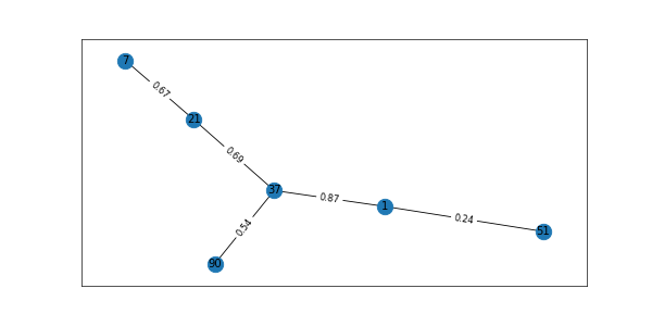
Interpreting the prediction. Refer code below. Our subgraph has labels for nodes 1,21,37,51 and for nodes 7 and 90 no labels are defined

H.nodes[1]['label'],G.nodes[21]['label'],G.nodes[37]['label'],G.nodes[51]['label']
# ('Machine Learning', 'NLP', 'Neural Network', 'Deep Learning')

Now refer the Subgraph H. from the figure, we can see that node 7 is attached to node 21 (NLP) and node 90 is attached to node 37 (Neural Networks) and the algorithm correctly predicted the missing node label as 1 (Machine Learning) – 21 (NLP) – 37 (Neural Networks) – 51 (Deep Learning) – 7 (NLP) – 90 (Neural Networks). Wow !!

Link Prediction 

In the link prediction, the algorithm gives the likelihood of future links getting attached to the graph with a probability score. Application of the link prediction could be identifying the friendship amongst users in social networking, identifying alternate routes in navigation, etc. networkx has multiple algorithms but in this article, I will talk about

Jaccard Coefficient:

This will give a similarity score for all pairs of nodes u,v and is defined as

|T(u)∩ t(v)| / |T(u)∪ T(v)|, where T(u) denotes the neighbors of u

Jaccard Coefficients will return all possible tuples (u, v, p) where p is the probability similarity of nodes u and v. higher the value of p, the more chances of link connection between them

Resource Allocation Index: 

This is another similarity score between pair of nodes u,v like the Jaccard Coefficient and is defined as

Σ 1 / |T(w)| where summation ranges for w ∈ T(u)∩ t(v)

Now, let us apply this to the entire graph G

lp = nx.jaccard_coefficient(G)
for u, v, p in lp:
  if p > 0.60 : # show only those possible nodes whose probability > 60%
    print(f"({u}, {v}) -> {p:.8f}")
#(27, 84) -> 0.66666667
lp = nx.resource_allocation_index(G)
for u, v, p in lp:
  if p > 0.60:
    print(f"({u}, {v}) -> {p:.8f}")
#(9, 90) -> 0.70000000
#(39, 100) -> 0.83333333

Next Step

The next step in graph data science is to do a similar analysis using advanced techniques like creating Node and Edge feature vectors, using GCN-Graph Convolutional Neural Network to predict the node classification and link prediction, and ontology to create domain-specific knowledge graphs that can be fed to a GCN, etc

Conclusion to Graph Data Science 

The key takeaways from this article are:

• Some of the most popular concepts from graph theory were explained
• Then we learned how to create a graph in python using the networkx library
• Next, common graph-related operations were performed and applied to our data
• Finally, some of the widely used pre-built graph algorithms from the networkx library were tested on our graph

Even though I used random graph data science to explain this post, many of these techniques can also be used with real business datasets. I enjoyed doing the analysis and writing this blog. I hope you too enjoyed my article on graph data science. If you are new to graph data science concepts, refer to the links below.

The media shown in this article is not owned by Analytics Vidhya and is used at the Author’s discretion.

PATTABHIRAMAN SRINIVASAN 31 Mar 2023