


Because of climate change, algae inundation has increased dramatically in the Caribbean Sea in recent years. It has yielded negative consequences on biodiversity, the local economy, and public health by releasing toxic gases that safety organizations need to carefully monitor and forecast. We will see how to predict the hydrogen sulfide (H₂S) emissions caused by algae grounding by leveraging multimodal data: time series, satellite data, and oceanic weather.
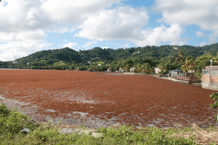 Sargassum Inundation in Martinique. Taken from Martinique Health Agency
This work has been carried out as part of a partnership between the Dataiku Lab and the Mediterranean Institute of Oceanography (MIO) in Toulon, France. We especially thank the co-authors of this work: Marine Laval, Cristele Chevalier, and Yamina Aimene.
Sargassum is a genus of macroalgae known for being the host of more than a hundred different fish and turtle species [1]. These free-floating algae sometimes constitute gigantic rafts extending over miles and serving as refuge and nursery for marine life.
However, since 2011, the Sargasso Sea — originally in the north of the Atlantic — has moved towards the equator following the modification of winds and currents induced by climate change [2,3]. In a warmer and more nutritive water, the algae have thrived and proliferated. This increase in algae biomass has led to more frequent and critical beach inundation also called “brown tides.”
This phenomenon has environmental consequences by trapping turtles and creating “dead zones” that asphyxiate other species. It also has economic implications by hindering the fishing and tourism industries. On top of that, Sargassum inundations pose important threats to local populations. Indeed, their decomposition releases various dangerous gases such H₂S which can cause nausea and vomiting [4] and can even provoke dangerous gestational disorders in pregnant women [5].
In this blog post, we will try to predict the Sargassum-induced H₂S emission by leveraging machine learning (ML) techniques. We will focus on predicting five days ahead to take into account the time needed to take action (i.e., move away pregnant women).
The Data at Our Disposal
H₂S Past Values
Over different stations around Martinique, H₂S is under the constant watch of sensors monitored by Madininair, an air quality organization. Its concentration is logged daily in ppm since 2018 and is publicly available.
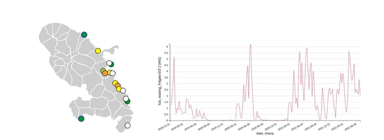 Map of the different air stations (left) and concentration of H₂S over time in one of them (right)
Over time, the concentration of H₂S can vary over a wide range from 0 up to 8 ppm. In addition, important variations in concentration can occur really fast over time with sudden peaks. Between October and March, the intensity of Sargassum inundation reduces and the H₂S concentrations are often near zero.
The concentration recorded by the different monitors also varies greatly over Martinique: Some stations are much less exposed than others to Sargassum inundations (because of the beach shape, for example) and will have low H₂S concentrations throughout the year.
Satellite Data From Sentinel Mission
The European Space Agency has developed seven satellite missions under the Sentinel program for land, ocean, and spectral monitoring. Each mission leverages a constellation of two satellites that embark different measurement instruments depending on its goal. Here, we focus on two different missions:
- Sentinel-2 (S2): Primarily designed for land monitoring, these satellites have a revisit frequency of five days, with a swath width of 290km and a resolution of 50m.
- Sentinel-3 (S3): Primarily designed for marine monitoring, these satellites have a daily revisit frequency, a swath width of 1270km, and a resolution of 300m.
However, this satellite data includes multiple instruments with many spectral bands and it is not an easy task to identify Sargassum rafts in it.
Some work has proposed index-based methods by computing metrics on different spectral bands [6,7,8]. Unfortunately, these methods can yield high false positive rates of up to 50% [9], and deep learning techniques have been investigated to overcome this issue [10,11].
The MIO used state-of-the-art architecture [12] to preprocess this satellite sentinel data (focusing around Martinique) and then provided us the images with identified Sargassum locations. These preprocessed images contain latitude and longitude information and are the ones used for training the models. In this blogpost we focus only on S2 images.
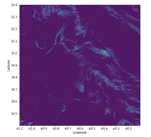 Sentinel-2 satellite data with Sargassum location
Oceanic Weather Data
In addition, to be able to better describe the Sargassum movement, we gathered data that describes the daily state of the ocean near Martinique:
- Current velocity from the Copernicus Marine System at a resolution of 1/12° (in latitude and longitude)
- Wave velocity from the same provider at a resolution of 1/5°
- Wind velocity from the ERA5 satellite at a resolution of 1/4°
Each of these velocities is divided into two variables for northward and eastward velocities. The oceanic weather is gathered around Martinique at the same latitude and longitude as the Sentinel satellite data.
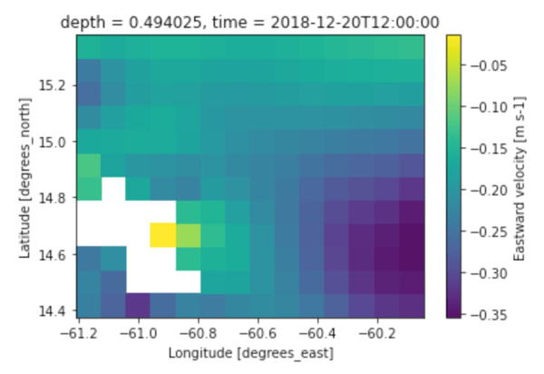 Eastward current velocity around Martinique
Tackling the Problem!
As this task has not yet been addressed by ML literature, we propose ML baselines for this specific task. We hope this work will make people aware of its complexity and eager to pursue it and other climate-related issues.
We train one unique model to predict for all stations in Martinique. We test three tree-based architectures: XGBoost, LightGBM, and Random Forest. We did a random search with 10 runs and 5-fold time-ordered cross-validation on the root-mean-squared-error (RMSE) to choose the best set of hyperparameters.
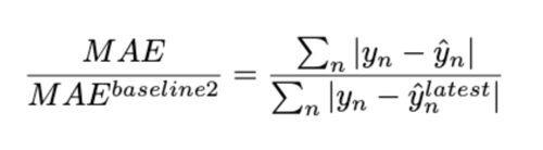
The two metrics used for comparing the models are the RMSE and MASE. The MASE (mean-absolute-scaled-error) is a scaled version of the mean-absolute error which can be computed for zero ground truth values, which are numerous in our data. It is expressed as the mean absolute error of the model divided by the mean absolute error of a baseline.
As a first approach, we can try to predict the value of H₂S at D+5 in a traditional time-series fashion. To this end we do some feature engineering on the sulfide concentration:
- Lagged features with 1 and 2 time-lags (H₂S at D-1 and D-2)
- Min, max, average, and standard deviation over rolling windows of different lengths (3/7/14 previous days)
- Similar windowed features but computed over all different stations of Martinique
In addition, to give some insights from the satellite data, we propose a simple density embedding by dividing each satellite image into a 3x3 grid and computing the total amount of Sargassum in each grid cell.
We are comparing our approach to two naive baselines for time series:
- Baseline 1: Compute the mean of the past values at the same date (meteorologic mean).
- Baseline 2: Use the last available value to predict H₂S in five days (D+5).
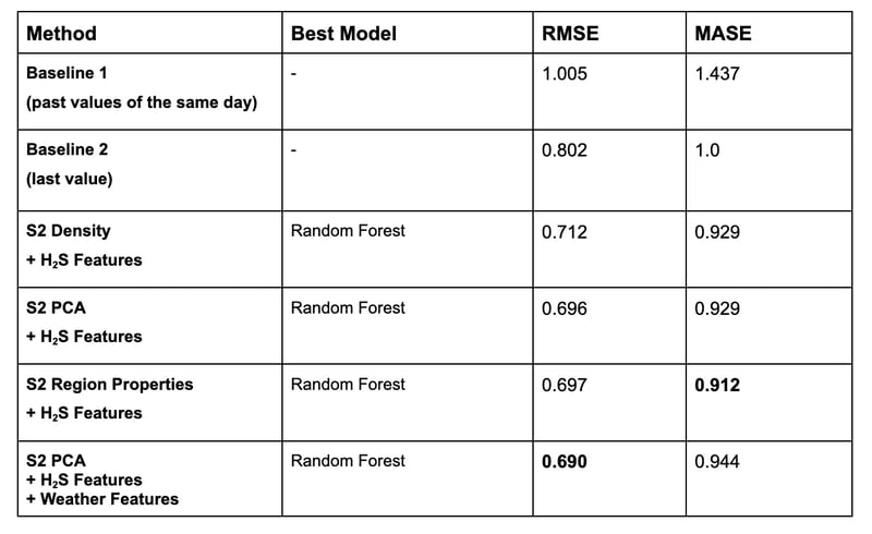
As this simple model already beats the baselines that we proposed (RMSE: 0.71 vs 0.8), it relies almost only on past H₂S values. On the one hand, even if the number of Sargassum that ground on the beaches should be directly linked to the H₂S emissions, the image embedding is underused. We need to find better ways to use Sargassum position information.
However, we cannot directly pass the satellite images to the model as they are huge (10k x 10k pixels) and not abundant enough (once a day for S3 and every five days for S2) to train an auto-encoder to reduce their dimension. Thus, we investigate other ways of reducing the dimension of our satellite data.
The first one is to compute the region properties of the Sargassum rafts. It can be done by detecting the ten largest connected regions in the S2 images using skimage (see below). Then, we can compute informative metrics on these regions such as the area, the bounding box coordinates, the centroid, the Euler number, or the orientation. In the end, each image is encoded in a set of a hundred different features (10 for each connected region).
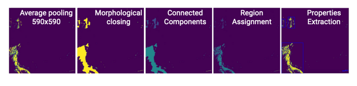 Region proporties extraction
The second method that we investigate and which is often used in dimensionality reduction is principal component analysis (PCA) which is often used on image data. As before, we reduce the S2 satellite images first to size (549,549) and then compute the PCA to retain 95% of the total variance of the images. This way, the satellite image can be represented by using only 102 principal components.
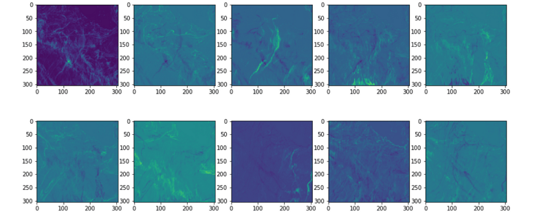 10 principal components of the PCA
Regarding the RMSE, the PCA approach yields better results (0.696 vs. 0.697), while the region properties approach is better in terms of MASE (0.912 vs. 0.929).
Finally, to increase the performance of our model even more, we incorporate weather data into the features. Indeed, knowing the Sargassum position should help the model but knowing where these Sargassums are going should help even more.
As for satellite images, we reduce the dimension of the weather data using PCA. One PCA is fitted for each type of weather data (wind, current, and wave velocity) and for each of the directions (northward and eastward) while retaining 95% of the total variance. We thus represent weather data as a set of 24 different features. In addition, as weather models give forecasting up to ten days, we compute a windowed average over 11 days (D-5 to D+5) for each of the components.
As models were plateauing regarding our metrics, adding averaged weather data was a critical step by allowing better performance and giving us our top-performing model. In addition, looking at the variable importance shows us that the model uses mainly the averaged values of weather data rather than the daily available value.
Here is a visual representation of models predictions over time:
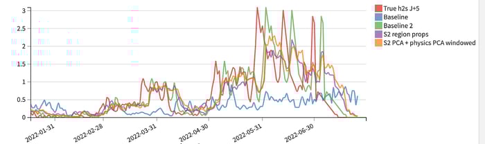 Comparison of different model predictions at D+5
Analysis
When looking at the variable importance of our best model, we observe that — even if the model still relies mostly on feature-engineered past values of H₂S — the importance of weather features accounts for 12% of the total. In addition, PCA-reduced satellite features, even if each individual feature importance is low, account for 11% percent of the total.
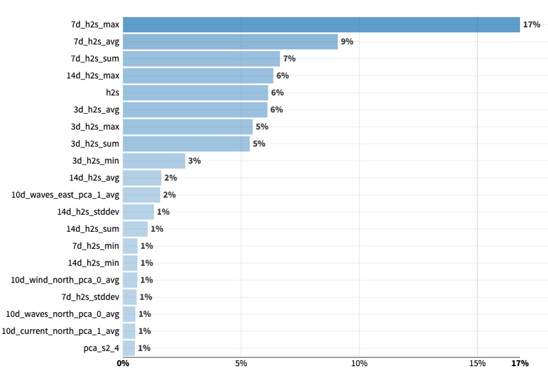 Most important variables of the best model
In addition, we observe that weather features are used more when predicting higher values of H₂S, while near-zero values rely almost exclusively on past H₂S values. This shows that the importance of weather data increases for rarer and more extreme cases.
We also observe that our model often underestimates peaks of H₂S which are more interesting to the task at hand because they are more dangerous for populations. This can be explained by the unbalanced data with many zero values (under detection threshold) and few high values in the training distribution.
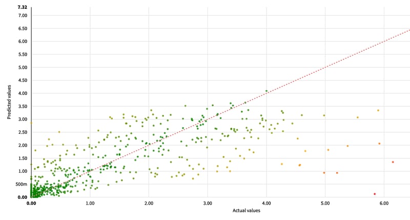 Error scatter plot
This analysis also shows us that it is difficult to predict a proxy of Sargassum inundation such as H₂S emission because it may involve both complex chemical and physical relations which are not easy to untangle.
Conclusion
We’ve shown how to leverage ML on multimodal data to mitigate one of the impacts of climate change. We’ve proposed the first ML baselines to the problem and are hoping that it can draw the gaze of the ML community upon it.
More globally, tackling and mitigating climate change opens a broad new range of applications of ML [12] from weather forecasting to smart grids and GHG emissions monitoring. However, knowledge in these domains tends to be siloed [14] and effort should be made to lower barriers between ML practitioners and subject matter experts.