It is good that there are no NULL values. And we need little changes in weight and Ram column to convert them to numeric by removing the unit written after value. So we will perform data cleaning here to get the correct types of columns.

data.drop(columns=['Unnamed: 0'],inplace=True)
## remove gb and kg from Ram and weight and convert the cols to numeric
data['Ram'] = data['Ram'].str.replace("GB", "")
data['Weight'] = data['Weight'].str.replace("kg", "")
data['Ram'] = data['Ram'].astype('int32')
data['Weight'] = data['Weight'].astype('float32')

EDA of Laptop Price Prediction Dataset

Exploratory analysis is a process to explore and understand the data and data relationship in a complete depth so that it makes feature engineering and machine learning modeling steps smooth and streamlined for prediction. EDA involves Univariate, Bivariate, or Multivariate analysis. EDA helps to prove our assumptions true or false. In other words, it helps to perform hypothesis testing. We will start from the first column and explore each column and understand what impact it creates on the target column. At the required step, we will also perform preprocessing and feature engineering tasks. our aim in performing in-depth EDA is to prepare and clean data for better machine learning modeling to achieve high performance and generalized models. so let’s get started with analyzing and preparing the dataset for prediction.

1) Distribution of target column

Working with regression problem statement target column distribution is important to understand.

sns.distplot(data['Price'])
plt.show()

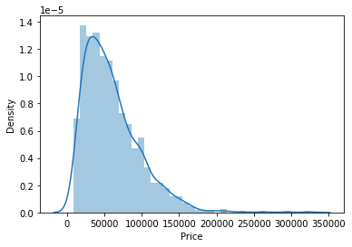
The distribution of the target variable is skewed and it is obvious that commodities with low prices are sold and purchased more than the branded ones.

2) Company column

we want to understand how does brand name impacts the laptop price or what is the average price of each laptop brand? If you plot a count plot(frequency plot) of a company then the major categories present are Lenovo, Dell, HP, Asus, etc.

Now if we plot the company relationship with price then you can observe that how price varies with different brands.

#what is avg price of each brand?

sns.barplot(x=data['Company'], y=data['Price'])

plt.xticks(rotation="vertical")

plt.show()

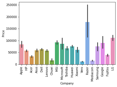
Razer, Apple, LG, Microsoft, Google, MSI laptops are expensive, and others are in the budget range.

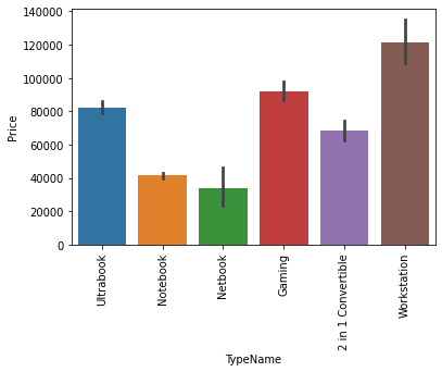
3) Type of laptop

Which type of laptop you are looking for like a gaming laptop, workstation, or notebook. As major people prefer notebook because it is under budget range and the same can be concluded from our data.

#data['TypeName'].value_counts().plot(kind='bar')
sns.barplot(x=data['TypeName'], y=data['Price'])
plt.xticks(rotation="vertical")
plt.show()

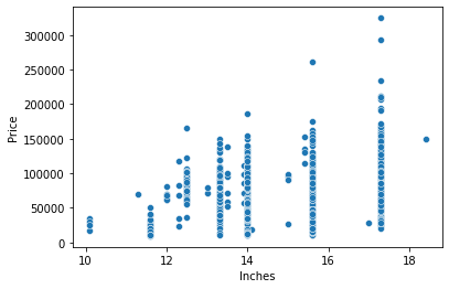
4) Does the price vary with laptop size in inches?

A Scatter plot is used when both the columns are numerical and it answers our question in a better way. From the below plot we can conclude that there is a relationship but not a strong relationship between the price and size column.

sns.scatterplot(x=data['Inches'],y=data['Price'])

Feature Engineering and Preprocessing of Laptop Price Prediction Model

Feature engineering is a process to convert raw data to meaningful information. there are many methods that come under feature engineering like transformation, categorical encoding, etc. Now the columns we have are noisy so we need to perform some feature engineering steps.

5) Screen Resolution

screen resolution contains lots of information. before any analysis first, we need to perform feature engineering over it. If you observe unique values of the column then we can see that all value gives information related to the presence of an IPS panel, are a laptop touch screen or not, and the X-axis and Y-axis screen resolution. So, we will extract the column into 3 new columns in the dataset.

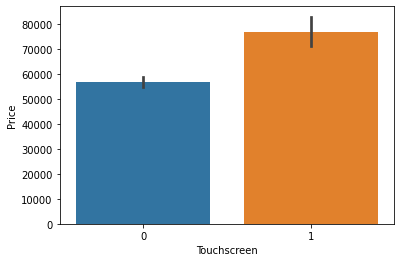
Extract Touch screen information

It is a binary variable so we can encode it as 0 and 1. one means the laptop is a touch screen and zero indicates not a touch screen.

data['Touchscreen'] = data['ScreenResolution'].apply(lambda x:1 if 'Touchscreen' in x else 0)
#how many laptops in data are touchscreen
sns.countplot(data['Touchscreen'])
#Plot against price
sns.barplot(x=data['Touchscreen'],y=data['Price'])

If we plot the touch screen column against price then laptops with touch screens are expensive which is true in real life.

Extract IPS Channel presence information

It is a binary variable and the code is the same we used above. The laptops with IPS channel are present less in our data but by observing relationship against the price of IPS channel laptops are high.

#extract IPS column
data['Ips'] = data['ScreenResolution'].apply(lambda x:1 if 'IPS' in x else 0)
sns.barplot(x=data['Ips'],y=data['Price'])

Extract X-axis and Y-axis screen resolution dimensions

Now both the dimension are present at end of a string and separated with a cross sign. So first we will split the string with space and access the last string from the list. then split the string with a cross sign and access the zero and first index for X and Y-axis dimensions.

def findXresolution(s):
  return s.split()[-1].split("x")[0]
def findYresolution(s):
  return s.split()[-1].split("x")[1]
#finding the x_res and y_res from screen resolution
data['X_res'] = data['ScreenResolution'].apply(lambda x: findXresolution(x))
data['Y_res'] = data['ScreenResolution'].apply(lambda y: findYresolution(y))
#convert to numeric
data['X_res'] = data['X_res'].astype('int')
data['Y_res'] = data['Y_res'].astype('int')

Replacing inches, X and Y resolution to PPI

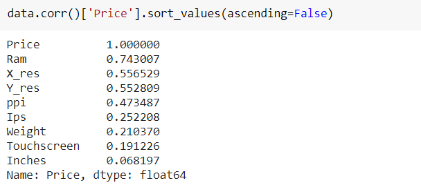
If you find the correlation of columns with price using the corr method then we can see that inches do not have a strong correlation but X and Y-axis resolution have a very strong resolution so we can take advantage of it and convert these three columns to a single column that is known as Pixel per inches(PPI). In the end, our goal is to improve the performance by having fewer features.

data['ppi'] = (((data['X_res']**2) + (data['Y_res']**2))**0.5/data['Inches']).astype('float')
data.corr()['Price'].sort_values(ascending=False)

Now when you will see the correlation of price then PPI is having a strong correlation.

So now we can drop the extra columns which are not of use. At this point, we have started keeping the important columns in our dataset.

data.drop(columns = ['ScreenResolution', 'Inches','X_res','Y_res'], inplace=True)

6) CPU column

If you observe the CPU column then it also contains lots of information. If you again use a unique function or value counts function on the CPU column then we have 118 different categories. The information it gives is about preprocessors in laptops and speed.

#first we will extract Name of CPU which is first 3 words from Cpu column and then we will check which processor it is
def fetch_processor(x):
  cpu_name = " ".join(x.split()[0:3])
  if cpu_name == 'Intel Core i7' or cpu_name == 'Intel Core i5' or cpu_name == 'Intel Core i3':
    return cpu_name
  elif cpu_name.split()[0] == 'Intel':
    return 'Other Intel Processor'
  else:
    return 'AMD Processor'
data['Cpu_brand'] = data['Cpu'].apply(lambda x: fetch_processor(x))

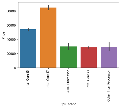
To extract the preprocessor we need to extract the first three words from the string. we are having an Intel preprocessor and AMD preprocessor so we are keeping 5 categories in our dataset as i3, i5, i7, other intel processors, and AMD processors.

How does the price vary with processors?

we can again use our bar plot property to answer this question. And as obvious the price of i7 processor is high, then of i5 processor, i3 and AMD processor lies at the almost the same range. Hence price will depend on the preprocessor.

sns.barplot(x=data['Cpu_brand'],y=data['Price'])
plt.xticks(rotation='vertical')
plt.show()

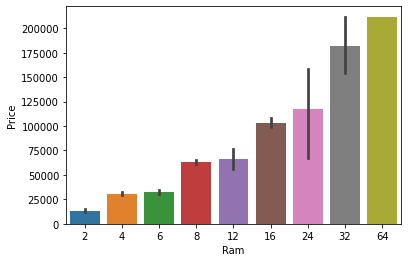
7) Price with Ram

Again Bivariate analysis of price with Ram. If you observe the plot then Price is having a very strong positive correlation with Ram or you can say a linear relationship.

sns.barplot(data['Ram'], data['Price'])
plt.show()

8) Memory column

memory column is again a noisy column that gives an understanding of hard drives. many laptops came with HHD and SSD both, as well in some there is an external slot present to insert after purchase. This column can disturb your analysis if not feature engineer it properly. So If you use value counts on a column then we are having 4 different categories of memory as HHD, SSD, Flash storage, and hybrid.

#preprocessing
data['Memory'] = data['Memory'].astype(str).replace('.0', '', regex=True)
data["Memory"] = data["Memory"].str.replace('GB', '')
data["Memory"] = data["Memory"].str.replace('TB', '000')
new = data["Memory"].str.split("+", n = 1, expand = True)
data["first"]= new[0]
data["first"]=data["first"].str.strip()
data["second"]= new[1]
data["Layer1HDD"] = data["first"].apply(lambda x: 1 if "HDD" in x else 0)
data["Layer1SSD"] = data["first"].apply(lambda x: 1 if "SSD" in x else 0)
data["Layer1Hybrid"] = data["first"].apply(lambda x: 1 if "Hybrid" in x else 0)
data["Layer1Flash_Storage"] = data["first"].apply(lambda x: 1 if "Flash Storage" in x else 0)
data['first'] = data['first'].str.replace(r'D', '')
data["second"].fillna("0", inplace = True)
data["Layer2HDD"] = data["second"].apply(lambda x: 1 if "HDD" in x else 0)
data["Layer2SSD"] = data["second"].apply(lambda x: 1 if "SSD" in x else 0)
data["Layer2Hybrid"] = data["second"].apply(lambda x: 1 if "Hybrid" in x else 0)
data["Layer2Flash_Storage"] = data["second"].apply(lambda x: 1 if "Flash Storage" in x else 0)
data['second'] = data['second'].str.replace(r'D', '')
#binary encoding
data["Layer2HDD"] = data["second"].apply(lambda x: 1 if "HDD" in x else 0)
data["Layer2SSD"] = data["second"].apply(lambda x: 1 if "SSD" in x else 0)
data["Layer2Hybrid"] = data["second"].apply(lambda x: 1 if "Hybrid" in x else 0)
data["Layer2Flash_Storage"] = data["second"].apply(lambda x: 1 if "Flash Storage" in x else 0)
#only keep integert(digits)
data['second'] = data['second'].str.replace(r'D', '')
#convert to numeric
data["first"] = data["first"].astype(int)
data["second"] = data["second"].astype(int)
#finalize the columns by keeping value
data["HDD"]=(data["first"]*data["Layer1HDD"]+data["second"]*data["Layer2HDD"])
data["SSD"]=(data["first"]*data["Layer1SSD"]+data["second"]*data["Layer2SSD"])
data["Hybrid"]=(data["first"]*data["Layer1Hybrid"]+data["second"]*data["Layer2Hybrid"])
data["Flash_Storage"]=(data["first"]*data["Layer1Flash_Storage"]+data["second"]*data["Layer2Flash_Storage"])
#Drop the un required columns
data.drop(columns=['first', 'second', 'Layer1HDD', 'Layer1SSD', 'Layer1Hybrid',
       'Layer1Flash_Storage', 'Layer2HDD', 'Layer2SSD', 'Layer2Hybrid',
       'Layer2Flash_Storage'],inplace=True)

First, we have cleaned the memory column and then made 4 new columns which are a binary column where each column contains 1 and 0 indicate that amount four is present and which is not present. Any laptop has a single type of memory or a combination of two. so in the first column, it consists of the first memory size and if the second slot is present in the laptop then the second column contains it else we fill the null values with zero. After that in a particular column, we have multiplied the values by their binary value. It means that if in any laptop particular memory is present then it contains binary value as one and the first value will be multiplied by it, and same with the second combination. For the laptop which does have a second slot, the value will be zero multiplied by zero is zero.

Now when we see the correlation of price then Hybrid and flash storage have very less or no correlation with a price. We will drop this column with CPU and memory which is no longer required.

data.drop(columns=['Hybrid','Flash_Storage','Memory','Cpu'],inplace=True)

9) GPU Variable

GPU(Graphical Processing Unit) has many categories in data. We are having which brand graphic card is there on a laptop. we are not having how many capacities like (6Gb, 12 Gb) graphic card is present. so we will simply extract the name of the brand.

# Which brand GPU is in laptop
data['Gpu_brand'] = data['Gpu'].apply(lambda x:x.split()[0])
#there is only 1 row of ARM GPU so remove it
data = data[data['Gpu_brand'] != 'ARM']
data.drop(columns=['Gpu'],inplace=True)

If you use the value counts function then there is a row with GPU of ARM so we have removed that row and after extracting the brand GPU column is no longer needed.

10) Operating System Column

There are many categories of operating systems. we will keep all windows categories in one, Mac in one, and remaining in others. This is a simple and most used feature engineering method, you can try something else if you find more correlation with price.

#Get which OP sys
def cat_os(inp):
    if inp == 'Windows 10' or inp == 'Windows 7' or inp == 'Windows 10 S':
        return 'Windows'
    elif inp == 'macOS' or inp == 'Mac OS X':
        return 'Mac'
    else:
        return 'Others/No OS/Linux'
data['os'] = data['OpSys'].apply(cat_os)
data.drop(columns=['OpSys'],inplace=True)

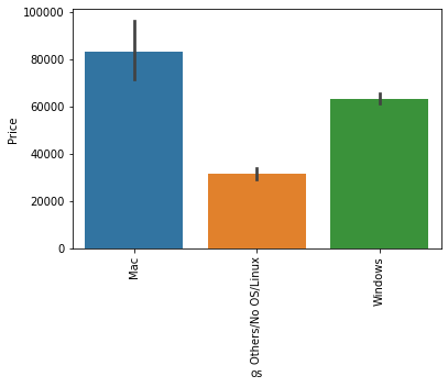
when you plot price aginst operating system then as usual Mac is most expensive.

sns.barplot(x=data['os'],y=data['Price'])
plt.xticks(rotation='vertical')
plt.show()

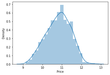
Log-Normal Transformation

we saw the distribution of the target variable above which was right-skewed. By transforming it to normal distribution performance of the algorithm will increase. we take the log of values that transform to the normal distribution which you can observe below. So while separating dependent and independent variables we will take a log of price, and in displaying the result perform exponent of it.

sns.distplot(np.log(data['Price']))
plt.show()

Machine Learning Modeling for Laptop Price Prediction

Now we have prepared our data and hold a better understanding of the dataset. so let’s get started with Machine learning modeling and find the best algorithm with the best hyperparameters to achieve maximum accuracy.

Import Libraries

from sklearn.model_selection import train_test_split
from sklearn.compose import ColumnTransformer
from sklearn.pipeline import Pipeline
from sklearn.preprocessing import OneHotEncoder
from sklearn.metrics import r2_score,mean_absolute_error
from sklearn.linear_model import LinearRegression,Ridge,Lasso
from sklearn.neighbors import KNeighborsRegressor
from sklearn.tree import DecisionTreeRegressor
from sklearn.ensemble import RandomForestRegressor,GradientBoostingRegressor,AdaBoostRegressor,ExtraTreesRegressor
from sklearn.svm import SVR
from xgboost import XGBRegressor

we have imported libraries to split data, and algorithms you can try. At a time we do not know which is best so you can try all the imported algorithms.

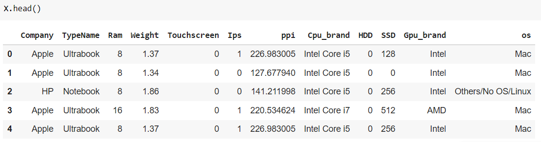
Split in train and test test

As discussed we have taken the log of the dependent variables. And the training data looks something below the dataframe.

X = data.drop(columns=['Price'])

y = np.log(data['Price'])

X_train,X_test,y_train,y_test = train_test_split(X,y,test_size=0.15,random_state=2)

 

Implement Pipeline for training and testing

Now we will implement a pipeline to streamline the training and testing process. first, we use a column transformer to encode categorical variables which is step one. After that, we create an object of our algorithm and pass both steps to the pipeline. using pipeline objects we predict the score on new data and display the accuracy.

step1 = ColumnTransformer(transformers=[

('col_tnf',OneHotEncoder(sparse=False,drop='first'),[0,1,7,10,11])

],remainder='passthrough')

step2 = RandomForestRegressor(n_estimators=100,

random_state=3,

max_samples=0.5,

max_features=0.75,

max_depth=15)

pipe = Pipeline([

('step1',step1),

('step2',step2)

])

pipe.fit(X_train,y_train)

y_pred = pipe.predict(X_test)

print('R2 score',r2_score(y_test,y_pred))

print('MAE',mean_absolute_error(y_test,y_pred))

In the first step for categorical encoding, we passed the index of columns to encode, and pass-through means pass the other numeric columns as it is. The best accuracy I got is with all-time favorite Random Forest. But you can use this code again by changing the algorithm and its parameters. I am showing Random forest. you can do Hyperparameter tuning using GridsearchCV or Random Search CV. we can also do feature scaling but it does not create any impact on Random Forest.

Exporting the Model

Now we have done with modeling. we will save the pipeline object for the development of the project website. we will also export the data frame which will be required to create dropdowns in the website.

import pickle
data.to_csv("df.csv", index=False)
pickle.dump(pipe,open('pipe.pkl','wb'))

Create Web Application for Deployment of Laptop Price Prediction Model

Now we will use streamlit to create a web app to predict laptop prices. In a web application, we need to implement a form that takes all the inputs from users that we have used in a dataset, and by using the dumped model we predict the output and display it to a user.

Streamlit

Streamlit is an open-source web framework written in Python. It is the fastest way to create data apps and it is widely used by data science practitioners to deploy machine learning models. To work with this it is not important to have any knowledge of frontend languages.

Streamlit contains a wide variety of functionalities, and an in-built function to meet your requirement. It provides you with a plot map, flowcharts, slider, selection box, input field, the concept of caching, etc. install streamlit using the below pip command.

pip install streamlit

create a file named app.py in the same working directory where we will write code for streamlit.

import streamlit as st
import pickle
import numpy as np
import pandas as pd
#load the model and dataframe
df = pd.read_csv("df.csv")
pipe = pickle.load(open("pipe.pkl", "rb"))
st.title("Laptop Price Predictor")
#Now we will take user input one by one as per our dataframe
#Brand
#company = st.selectbox('Brand', df['Company'].unique())
company = st.selectbox('Brand', df['Company'].unique())
#Type of laptop
lap_type = st.selectbox("Type", df['TypeName'].unique())
#Ram
ram = st.selectbox("Ram(in GB)", [2,4,6,8,12,16,24,32,64])
#weight
weight = st.number_input("Weight of the Laptop")
#Touch screen
touchscreen = st.selectbox("TouchScreen", ['No', 'Yes'])
#IPS
ips = st.selectbox("IPS", ['No', 'Yes'])
#screen size
screen_size = st.number_input('Screen Size')
# resolution
resolution = st.selectbox('Screen Resolution',['1920x1080','1366x768','1600x900','3840x2160','3200x1800','2880x1800','2560x1600','2560x1440','2304x1440'])
#cpu
cpu = st.selectbox('CPU',df['Cpu_brand'].unique())
hdd = st.selectbox('HDD(in GB)',[0,128,256,512,1024,2048])
ssd = st.selectbox('SSD(in GB)',[0,8,128,256,512,1024])
gpu = st.selectbox('GPU',df['Gpu_brand'].unique())
os = st.selectbox('OS',df['os'].unique())
#Prediction
if st.button('Predict Price'):
    ppi = None
    if touchscreen == "Yes":
        touchscreen = 1
    else:
        touchscreen = 0
    if ips == "Yes":
        ips = 1
    else:
        ips = 0
    X_res = int(resolution.split('x')[0])
    Y_res = int(resolution.split('x')[1])
    ppi = ((X_res ** 2) + (Y_res**2)) ** 0.5 / screen_size
    query = np.array([company,lap_type,ram,weight,touchscreen,ips,ppi,cpu,hdd,ssd,gpu,os])
    query = query.reshape(1, 12)
    prediction = str(int(np.exp(pipe.predict(query)[0])))
    st.title("The predicted price of this configuration is " + prediction)

Explanation – First we load the data frame and model that we have saved. After that, we create an HTML form of each field based on training data columns to take input from users. In categorical columns, we provide the first parameter as input field name and second as select options which is nothing but the unique categories in the dataset. In the numerical field, we provide users with an increase or decrease in the value.

After that, we created the prediction button, and whenever it is triggered it will encode some variable and prepare a two-dimension list of inputs and pass it to the model to get the prediction that we display on the screen. Take the exponential of predicted output because we have done a log of the output variable.

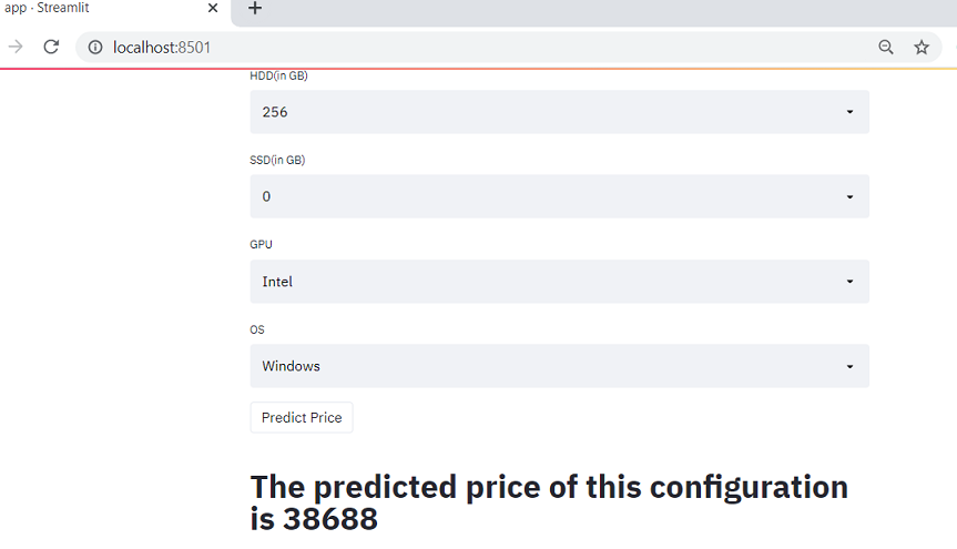
Now when you run the app file using the above command you will get two URL and it will automatically open the web application in your default browser or copy the URL and open it. the application will look something like the below figure.

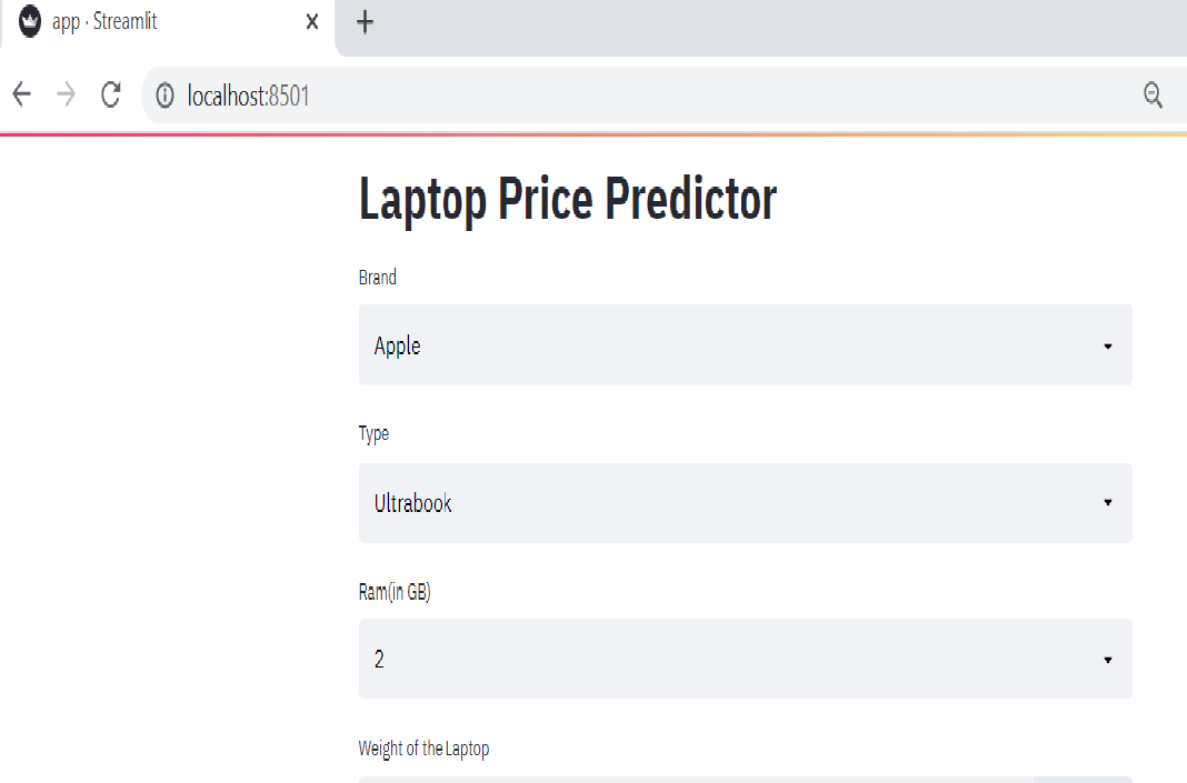
Enter some data in each field and click on predict button to generate prediction. I hope you got the desired results and the application is working fine.

Deploy Application to Heroku

Now we are ready to deploy our website and make it available for the public to use.

Prepare cloud files for deployment

1) Procfile

Create a file name Procfile which is an initiator file for Heroku. It only contains one line of code that says which file to run or it simply runs your python file.

web: sh setup.sh && streamlit run app.py

2) requirements

Create a file named requirements.txt. It is a text file that contains the name and version of a library that you have used to create your project. we need to define the libraries used to cloud so that when we deploy it creates a complete setup by installing required files. If you do not specify the version then it will install the current updated version of the library. we have used only four libraries for creating streamlit apps.

streamlit
sklearn
numpy
pandas

3) setup file

Create a file name setup.sh which contains how to create the directory structure in the cloud.

mkdir -p ~/.streamlit/
echo "
[server]n
port = $PORTn
enableCORS = falsen
headless = truen
n
" > ~/.streamlit/config.toml

Upload Code to Github

Log in to your GitHub account and create a new repository of the project name of your choice. Now you can either use the upload button to upload all files by selecting from a local file manager. And you can also use the GIT bash command as stated below to upload your code.

After creating a new repository copy the ssh link of a repository to connect with a repository. And then line by line follow the below commands.

git init #initialize empty repository
git remote add origin   #connect to repository
git pull origin master   #pull initial chnges
gid add -A #to add files in staging area
git commit -m initial commit
git push origin master  #push all files to github

Deploy to Heroku

Log in or register to Heroku if you do not have an account. After you log in in the top-right corner you will have the option of new. create a new app. Give a unique name to your code and this name will be your website URL followed by the Heroku domain and let the region be united states only.

Connect to repository

As you create an app, you will be redirected to the app dashboard. Now it’s time to connect Heroku to our Github repository. select Github and search your repository where you have pushed all application code and connect with it.

Deploy the code

Now scroll down and you have the option to deploy code. we will deploy on the main branch. Click on deploy branch and observe logs. After successfully deployment it will give you the web app URL on the view app option and your application is deployed successfully.

Now you can share the URL with anyone to use your application.

Live demo web app URL – Laptop Price predictor

Complete code files developed – GitHub

End Notes

Hurray! we have developed and deployed a machine learning application for the prediction of laptop price. We have learned about the complete machine learning project lifecycle with practical implementation and how to approach a particular problem. I hope that the particular article motivates and encourage you to develop similar more application to enhance your understanding of various methods and algorithms to use and twin with different parameters.

I hope that it was easy to follow up on this article. If you have any queries, suggestions, or feedback please feel free to post in the comment section.

About The Author

I am pursuing a bachelor’s in computer science. I am a data science enthusiast and love to learn, work in data technologies.

Connect with me on Linkedin

Check out my other articles here and on Blogspot

Thanks for giving your time!

Raghav Agrawal 19 Sep 2022

I am a final year undergraduate who loves to learn and write about technology. I am a passionate learner, and a data science enthusiast. I am learning and working in data science field from past 2 years, and aspire to grow as Big data architect.