Classify University as Private or Public using MLIB
This article was published as a part of the Data Science Blogathon.
Introduction to MLIB
This article will help solve the real-world problem of students classifying the university as a Private or a Public university based on the features we fed in the model that will be trained by various three methods, which we will discuss later. In a nutshell, PySpark library is involved as we will be working with its MLIB library (The machine learning library of PySpark).

About the Dataset
We are using the famous Private VS Public Universities dataset which has 17 features that will work as the dependent columns and a target column named Private (the categorical column which has “Yes” for Private and “No” for Public)
Here is a brief description of all the columns:
- Private is our target column which values, Yes/No to classify the university as private/public respectively.
- Apps are the number of applications received.
- Accept is the total number of applications received.
- Enroll number is the total number of students who enrolled.
- Top10per Pct. has all the students from the top 10% of High School.
- Top25perc Pct. has students from the top 20% of High School.
- F.Undergrad holds the total number of full-time undergraduates.
- P.Undergrad have several part-time undergraduates.
- The outstate column holds the number of out-of-station students.
- Room_board is the room costs.
- Books_estimated is the cost of the books.
- The Personal_estimated column stores the personal spending of students.
- PhD. Pct. holds the total number of PhD holder faculty.
- Terminal Pct. the column has the number of terminal holder faculty.
- S.F ratio stimulates the Student/Faculty Ratio.
- perc. alumni Pct. have the number of alumni who donate.
- Expend has the instructional expenditure of each student.
- Grad rates have the graduation rate values.
To achieve the aim of developing a good model for our problem statement we will be using various trees methods that are as follows:
- A single decision tree
- A random forest
- A gradient boosted tree classifier
Initializing the Spark Session
As we are well aware of the mandatory steps that we need to follow to start the spark session because for working with PySpark there should be all the resources available to us and setting up the environment is the key thing to do.
from pyspark.sql import SparkSession
spark = SparkSession.builder.appName('treecode').getOrCreate()
Inference: For initializing the session we imported the Spark object from the pyspark library. Then for creating the environment of Apache Spark we used the builder and the create function of the SparkSession object.
Reading the Dataset
Let’s read our dataset now from PySpark’s read.csv function so that we could then predict that according to the given features it is the Private college or the Public one.
Note: While we are passing the name of the dataset in the first parameter though note that in the second and third param i.e. inferSchema and header are set to True so that original types in the dataset should be shown.
data = spark.read.csv('College.csv',inferSchema=True,header=True)
data.show()
Output:
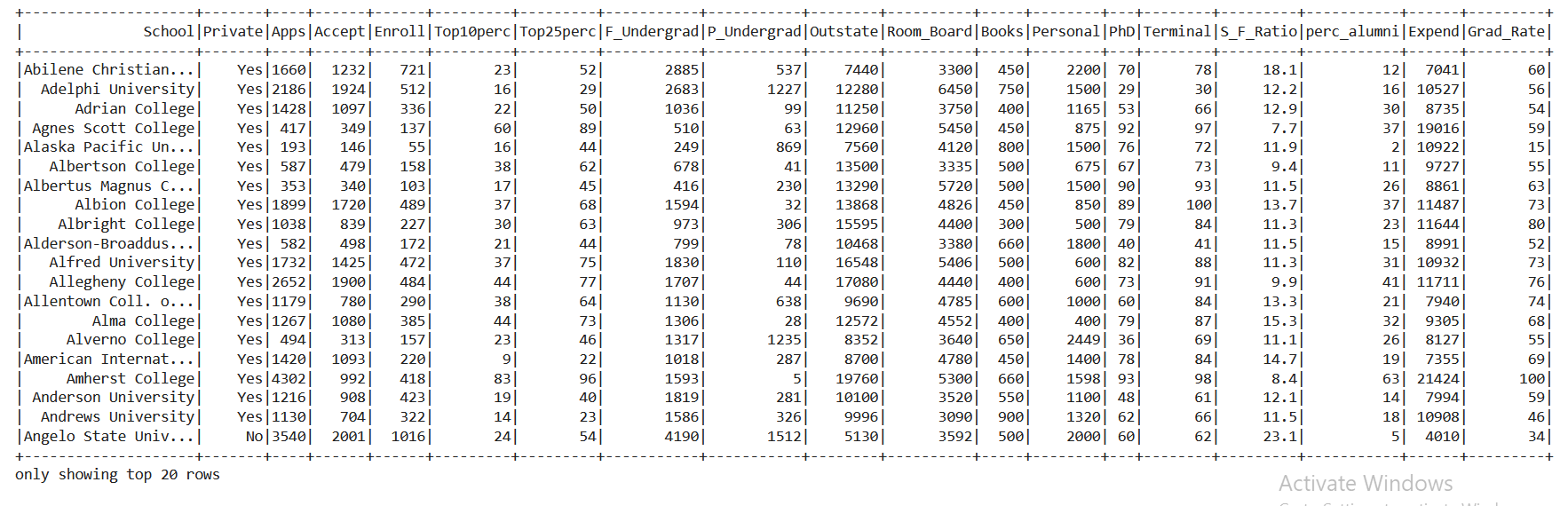 Inference: So in the output, it returned the complete data in the form of the dataset and showed up in the top 20 rows. Please have a note to our target column i.e. Private.
data.describe().show()
Output:
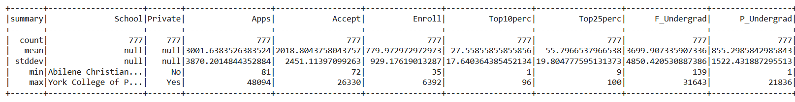
Inference: The described function of PySpark provides brief statistical information about the dataset which is quite informative. We can also see that the count of each column is the same i.e. 777 which stimulates there are no null values.
data.printSchema()
Output:
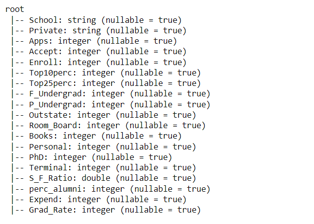
Inference: printSchema() is yet another function of PySpark where it gives us the complete information about the original Schema of the dataset along with that it returns the type of the data as well as nullable value (true/false) corresponding to the each feature.
data.head()
Output:
Row(School='Abilene Christian University', Private='Yes', Apps=1660, Accept=1232, Enroll=721, Top10perc=23, Top25perc=52, F_Undergrad=2885, P_Undergrad=537, Outstate=7440, Room_Board=3300, Books=450, Personal=2200, PhD=70, Terminal=78, S_F_Ratio=18.1, perc_alumni=12, Expend=7041, Grad_Rate=60)
Inference: Head method is yet another method to look into data more closely as along with showing the column name it also returns the value associated with it hence, becomes quite handy when we want to get more inference of what data it is constituting.
Formatting the Dataset
By far we are investigating the data like what type of data each feature is holding, is there any null values or not and stuff like that but now it’s time to format the dataset in such a way that it becomes capable enough to be fed to the machine learning algorithm.
There are a few mandatory things that we need to perform so that Spark MLIB could accept our data. It should have only two columns i.e. the label column which is the target one and the features column which holds the set of all features.
from pyspark.ml.linalg import Vectors
from pyspark.ml.feature import VectorAssembler
Inference: Here we are importing two of the main libraries that will help us to format the dataset that PySpark could accept which are Vectors and VectorAssembler.
data.columns
Output:
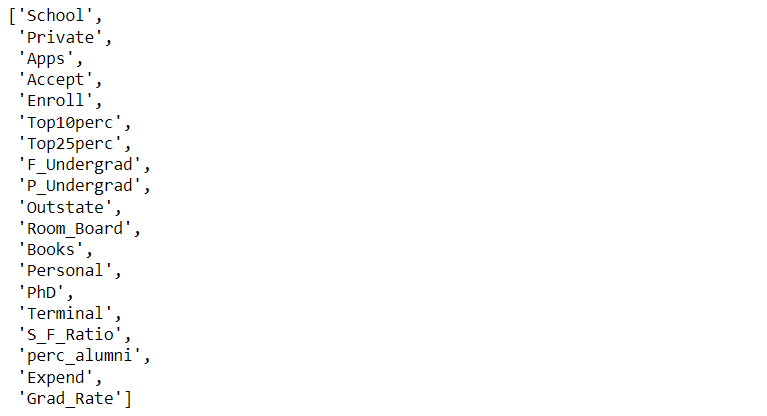
Inference: Whomsoever is following my PySpark series will notice that just before creating the assembler object I always used to see my data columns this helps me in saving time while typing the names hence one can either see the name of the features + target or can take it as a tip for efficient coding.
assembler = VectorAssembler(
  inputCols=['Apps',
             'Accept',
             'Enroll',
             'Top10perc',
             'Top25perc',
             'F_Undergrad',
             'P_Undergrad',
             'Outstate',
             'Room_Board',
             'Books',
             'Personal',
             'PhD',
             'Terminal',
             'S_F_Ratio',
             'perc_alumni',
             'Expend',
             'Grad_Rate'],
              outputCol="features")

output = assembler.transform(data)
Inference: So now as we were aware of the right columns to be chosen hence we can make our assembler object that will help to combine all the features and make it the right fit for MLIB’s format.
Don’t forget to transform it so that we can see the permanent changes in the newly created DataFrame.
Converting Type of Target column
Previously we saw that the Private column i.e. independent column has the values as Yes/No but we can’t feed this type of String data to the model hence we need to convert this string data to binary categorical values (0/1)
from pyspark.ml.feature import StringIndexer

indexer = StringIndexer(inputCol="Private", outputCol="PrivateIndex")
output_fixed = indexer.fit(output).transform(output)

final_data = output_fixed.select("features",'PrivateIndex')
Code breakdown:
- When we want to convert any string data type to integer categorical values then StringIndexer comes into action.
- StringIndexer object is created where the input column is there as the parameter that needs the name of the column to be converted. Again we also need to transform it to view the permanent changes in the data.
- At the last, we created a new DataFrame (final_data) that has a features column and a Private Index (converted target column).
Splitting the Dataset (Training/Testing)
This is one of the quite important steps in any machine learning pipeline as after splitting the whole dataset we have enough data for our training purpose as well enough data for the testing purpose as the validation of the model is equally important as training it.
train_data,test_data = final_data.randomSplit([0.7,0.3])
Inference: After the execution of the above cell we are left with 70% of the training data and 30% of the testing dataset which will eventually be used for validating the model.
Model Development Phase
So as we have separated our dataset and left with an independent training set of data. Now, with this, we will train our model with all the available tree methods like Decision tree, Gradient Boosting classifier, and Random forest classifier.
from pyspark.ml.classification import DecisionTreeClassifier,GBTClassifier,RandomForestClassifier
from pyspark.ml import Pipeline
Inference: Importing all the mentioned tree classifiers from the ml. classification library. Along with that Pipeline module is imported and this one is completely optional as I’ll personally suggest that use the pipeline way only when you are transforming the data multiple times and it needs a specific order of execution.
Now we have to create the object of each model i.e. all the three tree models and store it in a certain variable so that later one can easily fit (train) it.
dtc = DecisionTreeClassifier(labelCol='PrivateIndex',featuresCol='features')
rfc = RandomForestClassifier(labelCol='PrivateIndex',featuresCol='features')
gbt = GBTClassifier(labelCol='PrivateIndex',featuresCol='features')
Inference: From the above three lines of codes we can assure that each tree model is created one common thing is that each model has the same parameter i.e. label column and the features column
Note: Here we are using the default parameters to maintain the simplicity of the model though one can change that to fine-tune the model.
Now let’s train the model i.e. fit the models using the fit function of MLIB.
dtc_model = dtc.fit(train_data)
rfc_model = rfc.fit(train_data)
gbt_model = gbt.fit(train_data)
Note: When one will train all the three models together (in one cell) then one should patient enough as it will take some time (depending on one’s system configuration).
Evaluating and Comparing the Model
In this section, we will compare and evaluate each model simultaneously so that we could come to the conclusion which model has performed the best hence that particular model will be taken to the deployment phase.
dtc_predictions = dtc_model.transform(test_data)
rfc_predictions = rfc_model.transform(test_data)
gbt_predictions = gbt_model.transform(test_data)
Inference: For evaluating the model we need to transform each tree algorithm via testing data as the evaluation is only done based on the results that we get from the testing data.
There are various evaluation metrics available in PySpark we just have to figure out what we need at what point in time i.e. either Binary Classification Evaluator or Multi-class Evaluator.
from pyspark.ml.evaluation import MulticlassClassificationEvaluator
Inference: Here we acquired the Multi-class classification Evaluator as we wanna see the Accuracy of the model and one needs to know that in a classification problem if we are going with a Binary classification evaluator then Accuracy, Precision, and such other metrics we can’t access but with Multi-class we can.
# Select (prediction, true label) and compute test error
acc_evaluator = MulticlassClassificationEvaluator(labelCol="PrivateIndex", predictionCol="prediction", metricName="accuracy")
Inference: So we build the MulticlassClassificationEvaluator object where we passed the label column, and prediction column as well as the name of the metrics that we wanna see.
dtc_acc = acc_evaluator.evaluate(dtc_predictions)
rfc_acc = acc_evaluator.evaluate(rfc_predictions)
gbt_acc = acc_evaluator.evaluate(gbt_predictions)
Inference: To see the results evaluate method is used which needs the evaluated data (tree_model_predictions)
print("Here are the results!")
print('-'*50)
print('A single decision tree had an accuracy of: {0:2.2f}%'.format(dtc_acc*100))
print('-'*50)
print('A random forest ensemble had an accuracy of: {0:2.2f}%'.format(rfc_acc*100))
print('-'*50)
print('A ensemble using GBT had an accuracy of: {0:2.2f}%'.format(gbt_acc*100))
Output:
Here are the results!
--------------------------------------------------
A single decision tree had an accuracy of: 91.67%
--------------------------------------------------
A random forest ensemble had an accuracy of: 92.92%
--------------------------------------------------
A ensemble using GBT had an accuracy of: 91.67%
Inference: At the last, we printed the accuracy of each model and found out that the random forest ensemble is the best when it comes to this particular problem statement.
Conclusion to MLIB
This is the last section of the article where we will have a look at everything we did so far to classify the private and public universities i.e. from starting the SparkSession to evaluating the model and choosing the best model the brief conclusion will help you to understand the flow of the machine learning pipeline via PySpark’s MLIB.
- Firstly, as usual, we set up a hassle-free environment and read the college dataset to do the data analysis.
- Then we look into the data closely to understand what changes need to be done in the data preprocessing step and later updated it too according to the requirements.
- Then comes the turn of the model development phase where we build various tree models so that later we could compare and choose the best one.
- In the last section, we evaluated the model and concluded that the random forest ensemble model performed best on the testing data.
Here’s the repo link to this article. I hope you liked my article on Classify University as Private or Public using MLIB. If you have any opinions or questions on MLIB, then comment below.
Connect with me on LinkedIn for further discussion on MLIB or otherwise.
The media shown in this article is not owned by Analytics Vidhya and is used at the Author’s discretion.


