Advanced OpenCV: BGR Pixel Intensity Plots
This article was published as a part of the Data Science Blogathon.
Introduction
This is another article pertaining to the topic of Computer Vision in the Python Programming Language. This article picks us from our previous ones.
Up to this point in our advanced OpenCV tutorial, specifically focusing on our topic of Contrast, we have successfully:
- Understood the concept of Contrast.
- Understood the concept of Histogram Equalization.
- Implemented Contrast Enhancement on a GRAYSCALE image.
- Plotted the Pixel Histogram of a GRAYSCALE image.
However, as one may know, our world comprises color. Lots and lots of it. Now we shall attempt to analyze the contrast and pixel intensities of a color image, i.e., an image in which color channels are present. If you have not read through my previous articles on Computer Vision, kindly navigate to My Analytics Vidhya Profile.
To facilitate this particular advanced OpenCV learning experience, we shall make use of an image that may be downloaded from this link. Alternatively, you may save the image found below.

Source: WallpaperAccess
Understanding Color Images
If you remember correctly from our previous articles, we learned that advanced OpenCV utilizes the BGR color channels- Not the RGB. One will find that the Red and Blue color channels have been swapped.
As one may see in the above image, there are a plethora of colors that are eye-catching as well as visually appealing to the eye. These various shades of colors are the result of color channels that are being mixed.
There are three color channels present in this image:
- Blue.
- Green.
- Red.
It is through the presence and mixture of these colors that the secondary colors, and many others, belonging to the color spectrum can emerge.
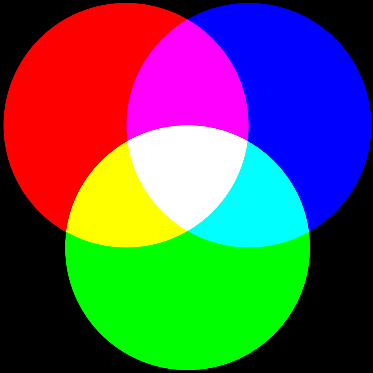
Source: Wikimedia Commons
Obtaining Image Insights
The first and foremost step would be to import the necessary packages into our python script, after which we then load the image into our system RAM. This will be accomplished using the imread() method available through the OpenCV package:
import cv2
import numpy as np
from matplotlib import pyplot as plt
img = cv2.imread('C:/Users/Shivek/Pictures/Picture1.jpg')
The output to the above code block will show as follows:

Source: WallpaperAccess
As one may observe, the image is too large to display on my screen in full size. However, we will NOT be reducing the size of the image. This is because we would like to gain insight into the properties of the Pixels and related information.
First, let us view the shape of the Image (NumPy array):
print(image.shape)
Output to the above line of code will show as follows:
Upon scrutinizing this tuple of information, one will decipher it as follows:
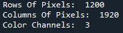
As we know, the color channel present is BGR- NOT RGB. Next, let us view the size of the Image– size tells us the total number of pixels that make up the entire image.
print(image.size)

There are over 6 million pixels in our image.
Let us view the first pixel in the image. This is the pixel in the first row, first column.
print(image[0][0])

It has a BGR value of 22, 15, and 6, respectively.
And now we move on to the portion we have all been waiting for; The BGR Pixel Count Plot.
The BGR Pixel Intensity Line Plot
Since each pixel in our image comprises 3 color channels, we are going to need to iterate through all pixels 3 times, each time picking out the values from the B, G, and R channels respectively. To perform this action it will be feasible to utilize a simple for loop in conjunction with the enumerate() function.
As we may already know, the enumerate() function will allow us to iterate through a fixed number of elements, and automatically keep a count of each.
We shall obtain a visual of the pixel intensities and counts, in the form of a line graph, using the MatPlotLib package.
colors = ('blue','green','red')
label = ("Blue", "Green", "Red")
for count,color in enumerate(colors):
    histogram = cv2.calcHist([image],[count],None,[256],[0,256])
    plt.plot(histogram,color = color, label=label[count]+str(" Pixels"))
Line-by-Line explanations of the above block of code are as follows:
In the below line of code, we have created a tuple comprising the colors for the three different lines of the graph. Since there are three iterations, upon each iteration a different color will be chosen, hence allowing for us to see the B-G-R patterns on the graph.
colors = (‘blue’, ‘green’, ‘red’)
We thereafter proceeded to create a tuple comprising corresponding labels for the legend of the graph. Again, upon each iteration, a label will be chosen to mark the corresponding color of the graph. These labels will be included in the legend of the graph, as we will see in a later line of code.
label = ("Blue", "Green", "Red")
To facilitate the graph generation, we have a for-enumerate loop that will be executed to select one of each required item from the array of pixels, and tuples, upon which they will be plotted as line graphs on the same canvas.
for count,color in enumerate(colors):
    histogram = cv2.calcHist([image],[count],None,[256],[0,256])
    plt.plot(histogram,color = color, label=label[count]+str(" Pixels"))
The line of code in the for-loop as shown below…
histogram = cv2.calcHist([image],[count],None,[256],[0,256])
…will make use of the calcHist() method from the OpenCV package, which will obtain a Histogram of pixel intensities, as we have learned in previous articles. We pass in the following parameters and arguments:
| Parameter | Argument |
| images= | [image] |
| channels= | [count] |
| mask= | None |
| histSize= | [256] |
| ranges= | [0, 256] |
To conclude the plotting of the graph, we make use of the plot() method offered by the MatPlotLib package as follows:
plt.plot(histogram, color=color, label=label[count]+str(" Pixels"))
We pass in the data to be plotted, followed by the appropriate color. We specify a label for the graph and index the corresponding label in the tuple according to the for-loop iteration. We append ” Pixels” to the label name to provide clarity to the viewer of the finished graph.
Before displaying the graph to the end-user, we add a few elements to the graph, such as:
- A Title.
- A Label for the Y-Axis.
- A Label for the X-Axis.
- A Legend.
To end the processing, we display the visual to the screen making use of the show() method offered by the MatPlotLib package.
plt.title("Histogram Showing Number Of Pixels Belonging To Respective Pixel Intensity", color="crimson")
plt.ylabel("Number Of Pixels", color="crimson")
plt.xlabel("Pixel Intensity", color="crimson")
plt.legend(numpoints=1, loc="best")
plt.show()
The final BGR Pixel intensity Line Plot will appear as follows:
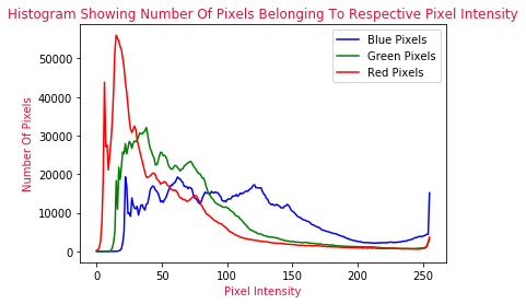
The above visualization shows and tells us exactly how the pixels are spread out in our original color image. The location of the 6 million+ pixels that make up our image, can be summarized in the above line plot.
Most of our pixels are found on the left of the image, and from the graph, one can expect the middle-to-right of the image to be blue in color, as indicated by the blue pixel intensity line. The blue pixel intensity line is dominant in these areas- which makes sense if one looks at the image:
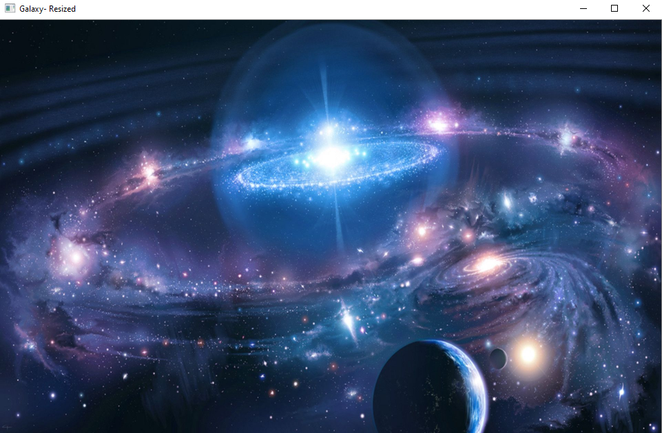
Notice how the full image fits on my computer screen- It is because I have resized it. A very interesting fact is that although I have resized the image if I were to create a pixel intensity plot on the resized image the gradient of the BGR plot would not at all differ when compared to the original- It will have just been reduced in size or “scale”.
Conclusion
This concludes my article on Advanced OpenCV: BGR Pixel Intensity Plots. I do hope that you have enjoyed reading through this article and have new takeaways from the OpenCV Package in Python Programming Language. In this article, we have looked at:
- Understanding color images with OpenCV in the Python Programming Language
- The BGR color channel
- Mapping BGR pixels to a BGR Pixel Intensity Line Plot using the MatPlotLib package in Python
Thank you for reading my article. Please feel free to connect with me on LinkedIn. I hope you have learned a new concept about advanced openCV With Python.
The media shown in this article is not owned by Analytics Vidhya and is used at the Author’s discretion.


