Introduction

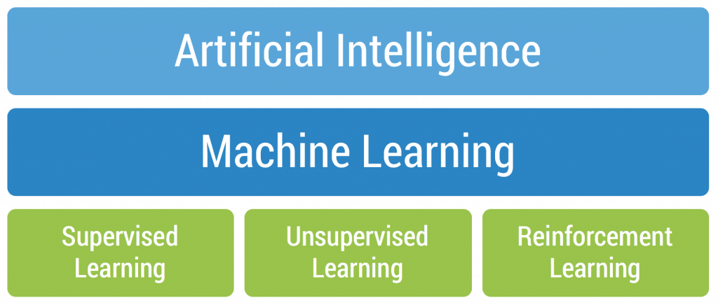
Reinforcement Learning (RL) can be defined as the study of taking optimal decisions utilizing experiences. It is mainly intended to solve a specific kind of problem where the decision making is successive and the goal or objective is long-term, this includes robotics, game playing, or even logistics and resource management.

In simple words, unlike the other machine learning algorithms, the ultimate goal of RL is not to be greedy all the time by looking for quick immediate rewards, rather optimize for maximum rewards over the complete training process. If you still wish to brush up on your knowledge of the reinforcement learning concepts, having a look at this glossary will really help!

Must-Know Terminologies Before Kicking Off This Topic

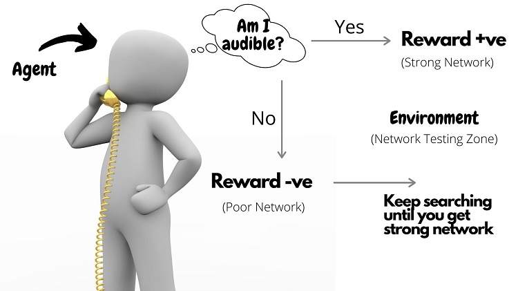
Agent:  The agent in RL can be defined as the entity which acts as a learner and decision-maker. It is empowered to interact continually, select its own actions, and respond to those actions.

Environment:  It is the abstract world through which the agent moves. The Environment takes the current state and action of the agent as input and returns its next state and appropriate reward as the output.

States:  The specific place at which an agent is present is called a state. This can either be the current situation of the agent in the environment or any of the future situations.

Actions:  This defines the set of all possible moves an agent can make within an environment.

Reward or Penalty:  This is nothing but the feedback by means of which the success or failure of an agent’s action within a given state can be measured. The rewards are used for the effective evaluation of an agent’s action.

Policy or Strategy:  It is mainly used to map the states along with their actions. The agent is said to use a strategy to determine the next best action based on its current state.

This article was published as a part of the Data Science Blogathon.

What is Q-learning?

Q-learning is a type of machine learning that helps a computer agent make decisions. It learns by trying different actions and determining which leads to the best results. Over time, the agent becomes smarter, making better choices based on gained experiences.

How did Q learning work?

Q-learning works by having an agent learn from its actions in an environment. The agent explores different actions, receives feedback on rewards or penalties, and adjusts its strategy to maximize cumulative rewards over time. This iterative process helps the agent make optimal decisions in various situations within the given environment.

The Q – Learning Algorithm in RL!

Of all the types of algorithms available in reinforcement learning, ever wondered why this Q-learning has always been the sought-after one? Here is the answer 😉

Q-learning is a model-free, value-based, off-policy learning algorithm.

• Model-free: The algorithm that estimates its optimal policy without the need for any transition or reward functions from the environment.
• Value-based: Q learning updates its value functions based on equations, (say Bellman equation) rather than estimating the value function with a greedy policy.
• Off-policy: The function learns from its own actions and doesn’t depend on the current policy.

Having known the basics, let’s now jump right away into the implementation part using simple python code. I suppose y’all would have gone through plenty of examples using the OpenAI baselines for illustrating different reinforcement learning algorithms.

Yet, this example can give you a clear-cut explanation about the exact working of the Q-learning algorithm in an effortless way!

Scenario – Robots in a Warehouse

A growing e-commerce company is building a new warehouse, and the company would like all of the picking operations in the new warehouse to be performed by warehouse robots.

• In the context of e-commerce warehousing, “picking” is the task of gathering individual items from various locations in the warehouse in order to fulfill customer orders.

After picking items from the shelves, the robots must bring the items to a specific location within the warehouse where the items can be packaged for shipping.

In order to ensure maximum efficiency and productivity, the robots will need to learn the shortest path between the item packaging area and all other locations within the warehouse where the robots are allowed to travel.

• We will use Q-learning to accomplish this task!

Import Required Libraries

#import libraries
import numpy as np

Define the Environment

The environment consists of states, actions, and rewards. States and actions are inputs for the Q-learning agent, while the possible actions are the agent’s outputs.

States

The states in the environment are all of the possible locations within the warehouse. Some of these locations are for storing items (black squares), while other locations are aisles that the robot can use to travel throughout the warehouse (white squares). The green square indicates the item packaging and shipping area.

The black and green squares are terminal states!

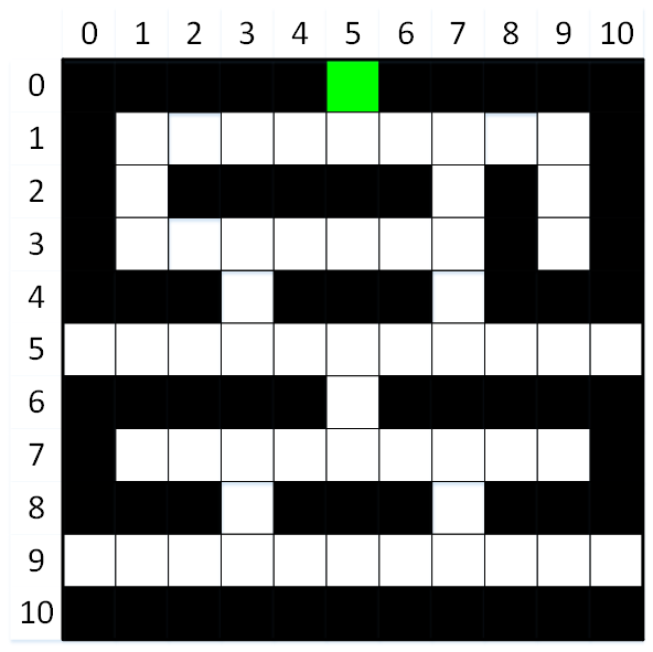
The agent’s goal is to learn the shortest path between the item packaging area and all of the other locations in the warehouse where the robot is allowed to travel.

As shown in the image above, there are 121 possible states (locations) within the warehouse. These states are arranged in a grid containing 11 rows and 11 columns. Each location can hence be identified by its row and column index.

Actions

The actions that are available to the agent are to move the robot in one of four directions:

• Up
• Right
• Down
• Left

Obviously, the agent must learn to avoid driving into the item storage locations (e.g., shelves)!

#define actions
#numeric action codes: 0 = up, 1 = right, 2 = down, 3 = left
actions = ['up', 'right', 'down', 'left']

Rewards

The last component of the environment that we need to define is the rewards. To help the agent learn, each state (location) in the warehouse is assigned a reward value. The agent may begin at any white square, but its goal is always the same: to maximize its total rewards! Negative rewards (i.e., punishments) are used for all states except the goal.

• This encourages the agent to identify the shortest path to the goal by minimizing its punishments!

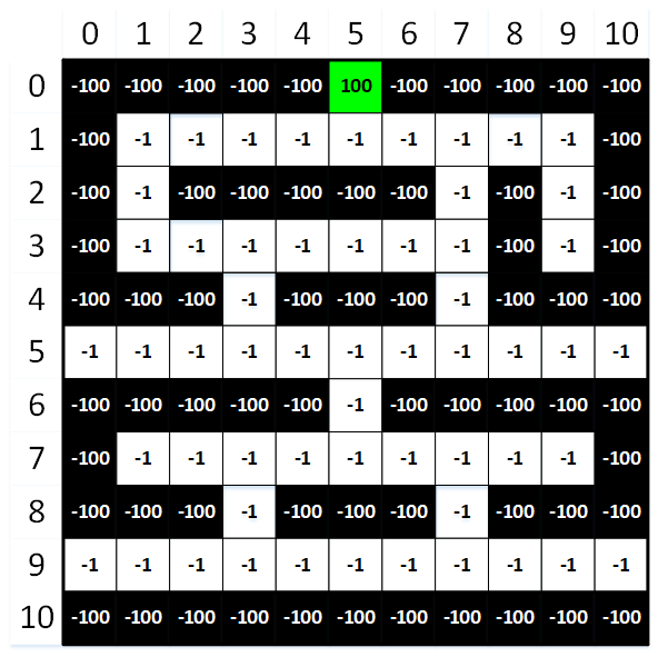
To maximize its cumulative rewards (by minimizing its cumulative punishments), the agent will need to find the shortest paths between the item packaging area (green square) and all of the other locations in the warehouse where the robot is allowed to travel (white squares). The agent will also need to learn to avoid crashing into any of the item storage locations (black squares)!

#Create a 2D numpy array to hold the rewards for each state. 
#The array contains 11 rows and 11 columns (to match the shape of the environment), and each value is initialized to -100.
rewards = np.full((environment_rows, environment_columns), -100.)
rewards[0, 5] = 100. #set the reward for the packaging area (i.e., the goal) to 100
#define aisle locations (i.e., white squares) for rows 1 through 9
aisles = {} #store locations in a dictionary
aisles[1] = [i for i in range(1, 10)]
aisles[2] = [1, 7, 9]
aisles[3] = [i for i in range(1, 8)]
aisles[3].append(9)
aisles[4] = [3, 7]
aisles[5] = [i for i in range(11)]
aisles[6] = [5]
aisles[7] = [i for i in range(1, 10)]
aisles[8] = [3, 7]
aisles[9] = [i for i in range(11)]
#set the rewards for all aisle locations (i.e., white squares)
for row_index in range(1, 10):
  for column_index in aisles[row_index]:
    rewards[row_index, column_index] = -1.
#print rewards matrix
for row in rewards:
  print(row)

Output:

[-100. -100. -100. -100. -100. 100. -100. -100. -100. -100. -100.] 
[-100. -1. -1. -1. -1. -1. -1. -1. -1. -1. -100.] 
[-100. -1. -100. -100. -100. -100. -100. -1. -100. -1. -100.] 
[-100. -1. -1. -1. -1. -1. -1. -1. -100. -1. -100.]
[-100. -100. -100. -1. -100. -100. -100. -1. -100. -100. -100.]
[-1. -1. -1. -1. -1. -1. -1. -1. -1. -1. -1.] 
[-100. -100. -100. -100. -100. -1. -100. -100. -100. -100. -100.] 
[-100. -1. -1. -1. -1. -1. -1. -1. -1. -1. -100.] 
[-100. -100. -100. -1. -100. -100. -100. -1. -100. -100. -100.] 
[-1. -1. -1. -1. -1. -1. -1. -1. -1. -1. -1.]
[-100. -100. -100. -100. -100. -100. -100. -100. -100. -100. -100.]

Train the Model

Our next task is for our agent to learn about its environment by implementing a Q-learning model. The learning process will follow these steps:

• Choose a random, non-terminal state (white square) for the agent to begin this new episode.
• Choose an action (move up, right, down, or left) for the current state. Actions will be chosen using an epsilon greedy algorithm. This algorithm will usually choose the most promising action for the agent, but it will occasionally choose a less promising option in order to encourage the agent to explore the environment.
• Perform the chosen action, and transition to the next state (i.e., move to the next location).
• Receive the reward for moving to the new state, and calculate the temporal difference.
• Update the Q-value for the previous state and action pair.
• If the new (current) state is a terminal state, go to #1. Else, go to #2.

This entire process will be repeated across 1000 episodes. This will provide the agent sufficient opportunity to learn the shortest paths between the item packaging area and all other locations in the warehouse where the robot is allowed to travel, while simultaneously avoiding crashing into any of the item storage locations!

Define Helper Functions

#define a function that determines if the specified location is a terminal state
def is_terminal_state(current_row_index, current_column_index):
  #if the reward for this location is -1, then it is not a terminal state (i.e., it is a 'white square')
  if rewards[current_row_index, current_column_index] == -1.:
    return False
  else:
    return True
#define a function that will choose a random, non-terminal starting location
def get_starting_location():
  #get a random row and column index
  current_row_index = np.random.randint(environment_rows)
  current_column_index = np.random.randint(environment_columns)
  #continue choosing random row and column indexes until a non-terminal state is identified
  #(i.e., until the chosen state is a 'white square').
  while is_terminal_state(current_row_index, current_column_index):
    current_row_index = np.random.randint(environment_rows)
    current_column_index = np.random.randint(environment_columns)
  return current_row_index, current_column_index
#define an epsilon greedy algorithm that will choose which action to take next (i.e., where to move next)
def get_next_action(current_row_index, current_column_index, epsilon):
  #if a randomly chosen value between 0 and 1 is less than epsilon, 
  #then choose the most promising value from the Q-table for this state.
  if np.random.random() < epsilon:
    return np.argmax(q_values[current_row_index, current_column_index])
  else: #choose a random action
    return np.random.randint(4)
#define a function that will get the next location based on the chosen action
def get_next_location(current_row_index, current_column_index, action_index):
  new_row_index = current_row_index
  new_column_index = current_column_index
  if actions[action_index] == 'up' and current_row_index > 0:
    new_row_index -= 1
  elif actions[action_index] == 'right' and current_column_index < environment_columns - 1:
    new_column_index += 1
  elif actions[action_index] == 'down' and current_row_index < environment_rows - 1:
    new_row_index += 1
  elif actions[action_index] == 'left' and current_column_index > 0:
    new_column_index -= 1
  return new_row_index, new_column_index
#Define a function that will get the shortest path between any location within the warehouse that 
#the robot is allowed to travel and the item packaging location.
def get_shortest_path(start_row_index, start_column_index):
  #return immediately if this is an invalid starting location
  if is_terminal_state(start_row_index, start_column_index):
    return []
  else: #if this is a 'legal' starting location
    current_row_index, current_column_index = start_row_index, start_column_index
    shortest_path = []
    shortest_path.append([current_row_index, current_column_index])
    #continue moving along the path until we reach the goal (i.e., the item packaging location)
    while not is_terminal_state(current_row_index, current_column_index):
      #get the best action to take
      action_index = get_next_action(current_row_index, current_column_index, 1.)
      #move to the next location on the path, and add the new location to the list
      current_row_index, current_column_index = get_next_location(current_row_index, current_column_index, action_index)
      shortest_path.append([current_row_index, current_column_index])
    return shortest_path

Train the Agent using Q-Learning Algorithm

#define training parameters
epsilon = 0.9 #the percentage of time when we should take the best action (instead of a random action)
discount_factor = 0.9 #discount factor for future rewards
learning_rate = 0.9 #the rate at which the agent should learn
#run through 1000 training episodes
for episode in range(1000):
  #get the starting location for this episode
  row_index, column_index = get_starting_location()
  #continue taking actions (i.e., moving) until we reach a terminal state
  #(i.e., until we reach the item packaging area or crash into an item storage location)
  while not is_terminal_state(row_index, column_index):
    #choose which action to take (i.e., where to move next)
    action_index = get_next_action(row_index, column_index, epsilon)
    #perform the chosen action, and transition to the next state (i.e., move to the next location)
    old_row_index, old_column_index = row_index, column_index #store the old row and column indexes
    row_index, column_index = get_next_location(row_index, column_index, action_index)
    #receive the reward for moving to the new state, and calculate the temporal difference
    reward = rewards[row_index, column_index]
    old_q_value = q_values[old_row_index, old_column_index, action_index]
    temporal_difference = reward + (discount_factor * np.max(q_values[row_index, column_index])) - old_q_value
    #update the Q-value for the previous state and action pair
    new_q_value = old_q_value + (learning_rate * temporal_difference)
    q_values[old_row_index, old_column_index, action_index] = new_q_value
print('Training complete!')

Output:

Training complete!

Get Shortest Paths

Now that the agent has been fully trained, we can see what it has learned by displaying the shortest path between any location in the warehouse where the robot is allowed to travel and the item packaging area.

Try out a few different starting locations!

#display a few shortest paths
print(get_shortest_path(3, 9)) #starting at row 3, column 9
print(get_shortest_path(5, 0)) #starting at row 5, column 0
print(get_shortest_path(9, 5)) #starting at row 9, column 5

Output:

[[3, 9], [2, 9], [1, 9], [1, 8], [1, 7], [1, 6], [1, 5], [0, 5]]

[[5, 0], [5, 1], [5, 2], [5, 3], [4, 3], [3, 3], [3, 4], [3, 5], [3, 6], [3, 7], [2, 7], [1, 7], [1, 6], [1, 5], [0, 5]]

[[9, 5], [9, 6], [9, 7], [8, 7], [7, 7], [7, 6], [7, 5], [6, 5], [5, 5], [5, 6], [5, 7], [4, 7], [3, 7], [2, 7], [1, 7], [1, 6], [1, 5], [0, 5]]

Finally…

It’s great that our robot can automatically take the shortest path from any ‘legal’ location in the warehouse to the item packaging area. But what about the opposite scenario?

Put differently, our robot can currently deliver an item from anywhere in the warehouse to the packaging area, but after it delivers the item, it will need to travel from the packaging area to another location in the warehouse to pick up the next item!

Don’t worry — this problem is easily solved simply by reversing the order of the shortest path!

#display an example of reversed shortest path
path = get_shortest_path(5, 2) #go to row 5, column 2
path.reverse()
print(path)

Output:

[[0, 5], [1, 5], [1, 6], [1, 7], [2, 7], [3, 7], [3, 6], [3, 5], [3, 4], [3, 3], [4, 3], [5, 3], [5, 2]]

Conclusion

I believe you had gained a basic yet vivid understanding of this Q – learning algorithm. There’s still a lot more for you to learn and experiment with! So just stay the course! Try on with your own scenarios and illustrations. I’ve added a few interesting resources below for you to begin with.

Resources

1. Reinforcement Learning: An Introduction – Richard S. Sutton and Andrew G. Barto.
2. David Silver’s lectures on RL.
3. RL Tutorial using Q – learning.
4. Q – learning Numerical Example.

The media shown in this article are not owned by Analytics Vidhya and is used at the Author’s discretion.

Frequently Asked Questions?