


It’s been four years since the last World Cup in 2018, when France won their second star on their crest. Even if you are not particularly interested in football, you might still find that World Cups are a fun moment where people share joy and excitement. I wanted to participate, but my knowledge would be limited to knowing Neymar and Kylian Mbappé's names. So as a data scientist by day, I knew that one way I could get involved was by building a machine learning (ML) model.

As the World Cup is approaching, we decided to create a team of the finest data scientists at Dataiku and work together to try to come up with a prediction (both the outcome and the exact scores) for the 64 games that will take place during the tournament.
Trying to forecast something as unpredictable as a sports outcome sounded fun (and very hard), but we went for it anyway. Using Dataiku, we created several competing models with different strategies, so be sure to follow along in this blog post (intended for rather technical practitioners) if you want to see how we did it — and who we have predicted to win!
Do We Really Need a Model to Know That Brazil Is the Favorite to Win?
If we aim at predicting only the final World Cup winner, the natural and safe choice is to bet for the favorite, Brazil, who is the No. 1 team in the FIFA World Rankings, already five-time world champions, and listed as the 4-1 favorites in the World Cup odds, according to NBC Sports). Too easy, isn’t it? And we all know that surprises can happen in football.
Instead, we put in place a traditional bookmakers set up. For each game, each outcome has an odd associated function of the likelihood of this outcome, that determines our potential gain. Let’s take the example of the France - Australia game. There are three possible outcomes: France winning, Australia winning, or a draw at the end of the 90 minutes.
Your ML model predicts the winner with an associated probability. If you solely consider the predicted probability, you would for sure bet on France (63% probability). However, if you take into account the odds, you realize that the expected gain you get by multiplying the probability by the odds in points format is higher for the Draw outcome. Therefore, you might want to take some calculated risk here and bet for the Draw outcome, as the expected gain is greater.
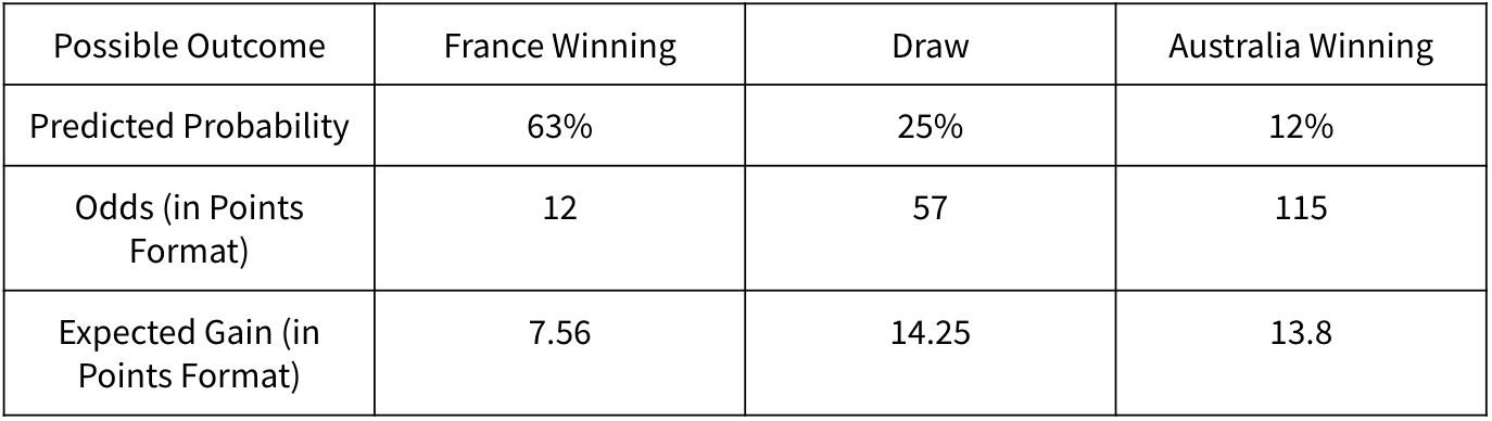
Probabilities, odds and expected gains for the France - Australia game
So now our model has actually two missions:
- Predict the outcome that maximizes the expected gain for each game (so not necessarily betting for the team most likely to win)
- Predict the correct score for each team, which can have a very significant impact. In our game, when you guess the correct scoreline, you double the points associated with the correct outcome guess. So for example in the France - Australia example detailed above, our model would predict a Draw to try to gain 57 points, but if we guess the correct scores (e.g., 1-1), we would actually win 114 points!
What data did we use to build this model?
Setting Technical Context
Understanding the Data
The dataset we used provides a complete overview of all international soccer matches played since the 1990s. It includes 23,921 matches from different tournaments that range from FIFA World Cup to regular friendly matches. The strength of each team is provided by FIFA rankings.
Each match is described with its context and characteristics of both teams:
- The date, tournament, location (country, city, neutral pitch or not), match outcome (win / draw / loss), and the scores of each team.
- The FIFA ranking (global, offense, defense, and midfield rankings). This method of ranking national teams takes into account international matches played over the course of four years and raises successful teams to the top of the ranking.
The team-related columns come with a prefix home or away indicating the location of the match. However, some matches (e.g., international competitions) are played in a neutral location. This information can be found in the boolean column neutral_location.
Exploring/Preparing the Data
First, the distribution of match outcomes show to be different between home/away and neutral locations. Naturally, the ratio of win/loss is in favor of the home team. Playing at home represents an obvious advantage and so biases the match outcome.
However, the ratio win/loss is surprisingly not equal to one when the location is neutral. This might bias a strategy modeling home/away scores as two independent variables. Restructuring the dataset should be considered, meaning removing home/away distinction and, for example, replacing it with a variable location taking home/away/neutral as values.
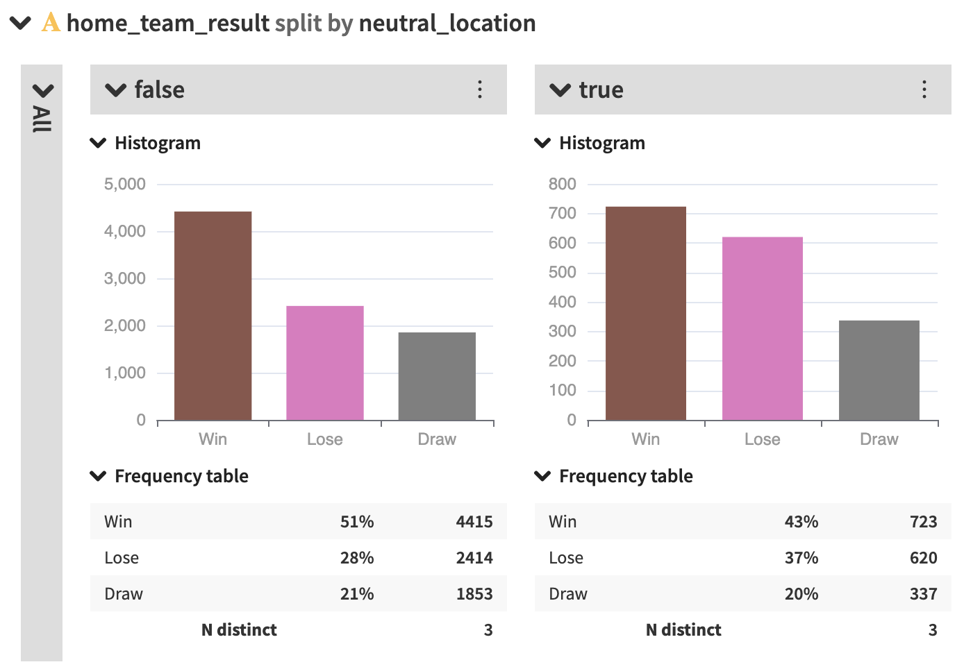
Distribution of match outcomes depending on their location (home/away or neutral)
Home and away team scores are the variables to be predicted. Somehow, the target variable must be understood as the joint distribution of home_score and away_score. And so it might be more convenient to describe matches by the two variables home + away and home - away scores, which both take into account the interaction between the teams (for the purpose of data exploration).
One of the main distinctive features of the FIFA World Cup is that it gathers the top teams of each continent. Meaning the train/test data has to be made of matches whose average level is representative of the World Cup's (for example, matches between two very low rated teams will be excluded).
Similarly to the variable score, we consider the “joint ranking” of the teams through the difference and sum of their ranks.
- The ranking difference has the same distribution over time for the FIFA World Cup, meaning past events are similar to most recent ones. They can be used equally as inputs of the model then.
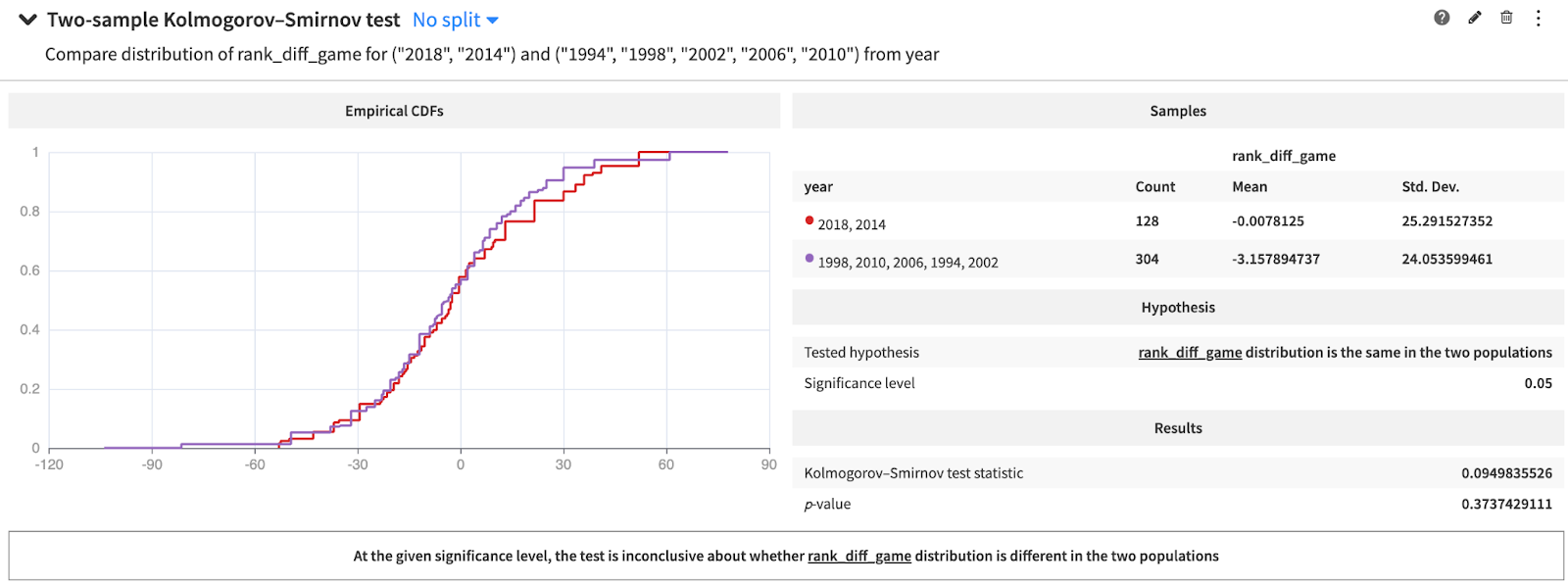
Distribution of match ranking compared between recent (2014 and 2018) and past (before 2014) World Cups
- The variable ranking difference is the top variable correlated with the number of goals, meaning it could be used to create a dataset representative of the World Cup matches. The distribution of the ranking difference lets us filter out the dataset: matches out of the "bounds" of the distribution are removed. These “bounds” are defined as the first and last percentiles and used to exclude some matches (seen as outliers) unlikely to happen, for example Korean DPR (105th) versus Brazil (1st) played in 2010-06-15 (which ended up with a surprising 1-2).
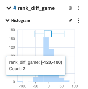
Distribution of team ranking difference in historical World Cup matches
- Similarly, the variable tournament is used to create a rank difference distribution similar to the World Cup's and retain "high stakes" matches. Indeed, competitions are not played with the same level of intensity as friendly matches. The distribution of ranks might differ between the World Cup and the other tournaments. Meaning matches not representing World Cup's level can be put aside in train/test sets. At the end, it is a compromise between the dataset size, the metrics and their reliability.
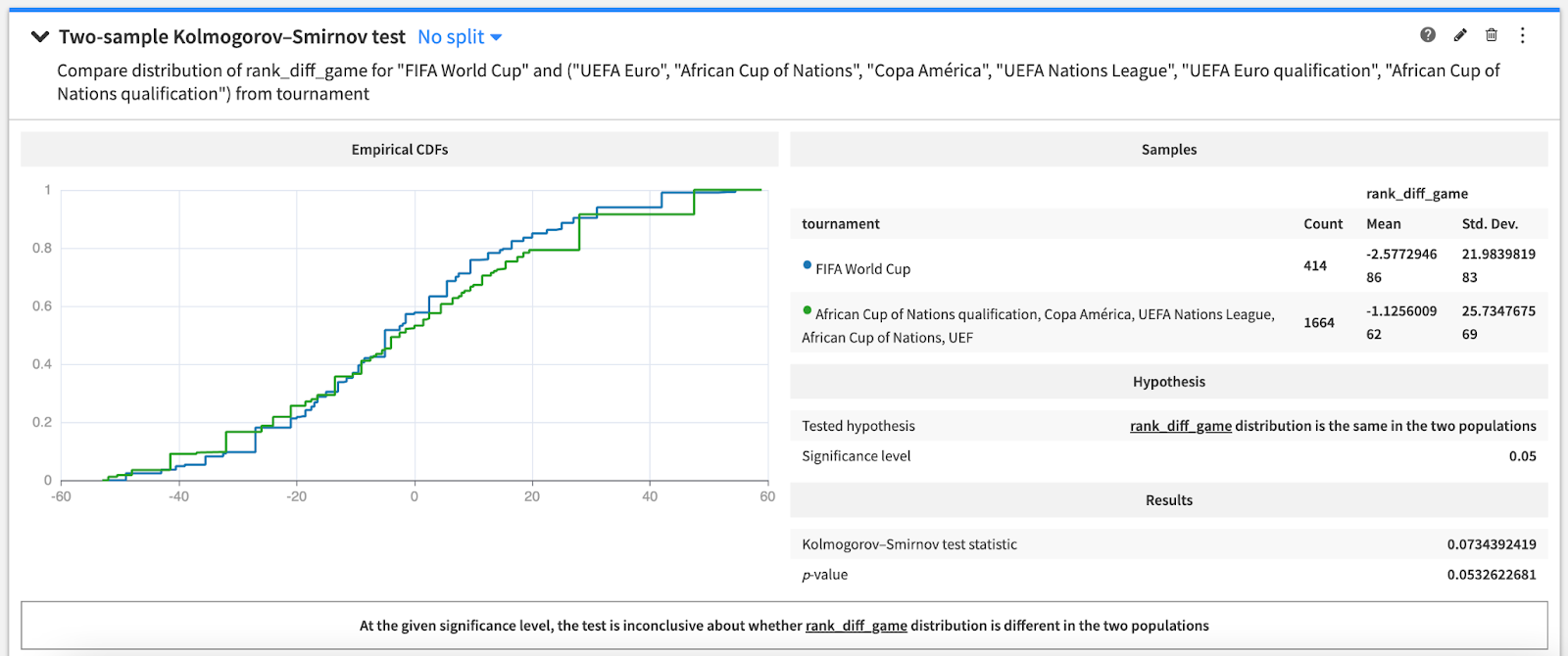
Kolmogorov-Smirnoff test showing the ranking of teams in the selected tournaments is similar to the World Cup’s
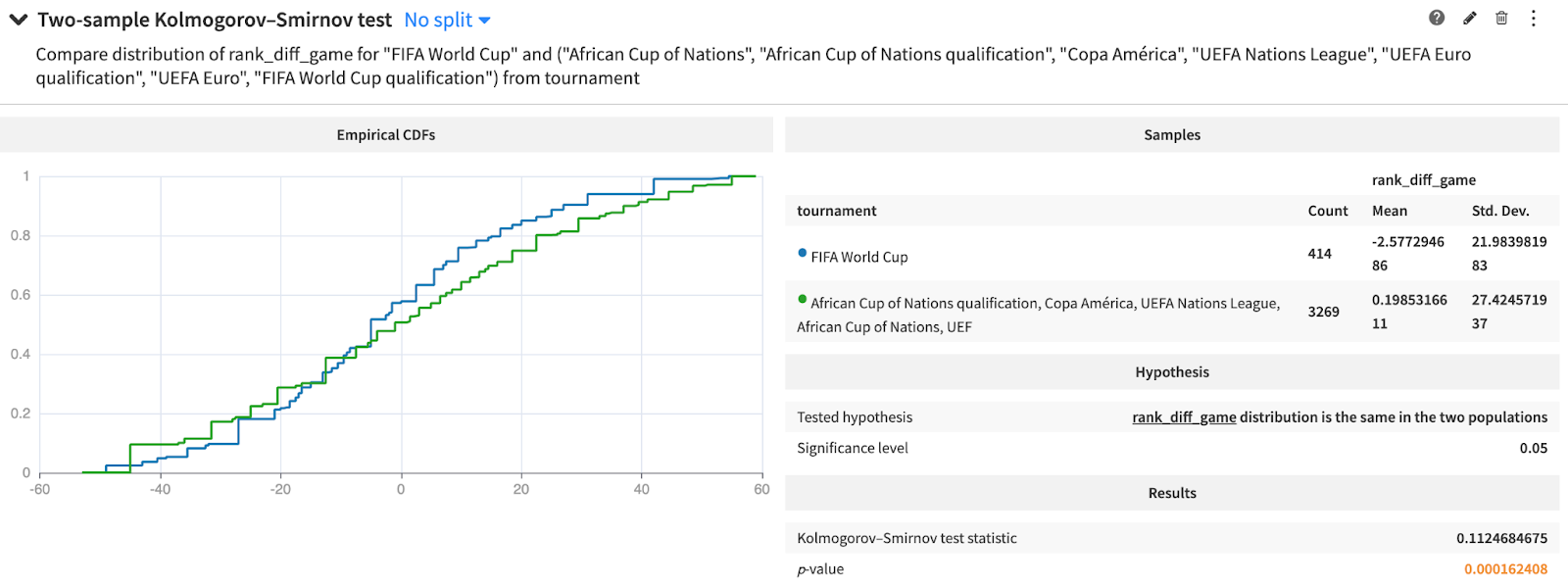
However, introducing the FIFA World Cup qualifications make the ranking distribution statistically different from the World Cup’s.
However, keep in mind that limiting matches to a given scope does not prevent the features generated to take into account other matches, such as preparatory matches.
Last but not least, the target variable can be used to remove unlikely matches from the dataset, typically matches with a number of goals exceeding the maximum ever observed in a World Cup, which is 8. This value could even be taken lower as we did with the ranking difference, if we believe values above a certain threshold might harm the model performance.
Defining a "Good" Model
How can we determine “good” models and compare them?
- For the first model, ideally we would want to create a model that maximizes the expected gain: odds (in points format) x predicted probability. However, we don’t have the historical odds. We decided to stick to a multi-class classification model, with the three classes being win, lose, draw. From a sports betting model perspective, we need to calibrate the model to get probabilities sensible enough for maximizing the expected gain. From a ML model perspective, the accuracy score needs to be maximized (basically the proportion of correct predictions).
- For the second model, we are looking to predict the correct score of both teams. There are different strategies here, either consider it as a multi-output regression, or have two independent regression models for each team score, and combine them. Both strategies would be possible, but we chose to go for the second one.
With the data exploration findings in mind, we filtered on matches from high stakes tournaments involving teams with a level similar to the World Cup’s. We performed a temporal split, keeping 75% of data for train and 25% for test.
Now that we have the right set up to evaluate our models, let’s dig into them. In the following section, we will introduce a first strategy based on a traditional approach combining different ML models.
Modeling Approach Based on Classical ML
Data Preparation
As explained before, the first step was to deal with the game location, to eliminate the potential bias associated with the feature. We went from having a dataset with one row per game, with one feature indicating the location (neutral or not), to a dataset having two rows per game.
But how did we create this second row? We actually duplicated the original row and swapped all the team features. It was also necessary to modify the location column, from being neutral or not to home / away / neutral.

Duplicating and swapping each game, Japan - Brazil example
Then, we created several features reflecting the dynamic of the teams preceding each game with temporal window functions. We chose two different frames, first the last year preceding each game, and then the last 10 games before each game in which we calculated:
- The average number of goals scored and conceded
- Their ratio of wins, losses and draws
Predicting the Game Outcome
The first stage is to predict the match outcome. As explained before, we can express that as a multi-class classification problem for the home team result, with three classes: Win, Draw or Lose.
We compared several models of different nature (logistic regression, random forest, XGBoost, and even k-nearest neighbors), optimizing the accuracy score. Despite our dataset being quite balanced (the distribution of the three classes is close to being even) our random forest was very good at predicting the Win and Lose classes, but much less so for the Draw one. We decided to continue with the random forest.

Performance (accuracy score) on compared algorithms
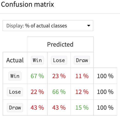
Confusion matrix for the random forest algorithm
After selecting the outcome maximizing the potential gain (cf. The France - Australia example detailed in the introduction), taking into consideration both the likelihood of the outcome and the associated odds (in points format), we could then use these outcomes to predict the scores of the two teams, which obviously need to be consistent with the predicted outcome.
Predicting the Score of Each Team
After predicting the game outcome, the second step of our approach was to predict the correct scoreline of each game. As introduced above, we chose to use two regression models, one for the Home team score and the other one for the Away team score.
For these two regression tasks, we once again compared the same models (but regressor versions), trying to minimize the Root Mean Squared Error this time. For both regression tasks, the random forest model ended up being the best one. Finally, we round the predictions to the closest integer and obtain a score for each team. Most important point: These scores are always consistent with the predicted outcome that was obtained in the previous classification step.
We then proceeded with scoring the first round of the group games, involving 16 games, and obtained to following predictions:
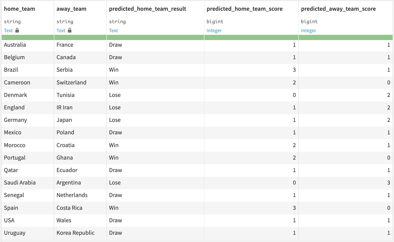
First round of predictions using the optimizing gain approach
For those who are familiar with football, some of these results might seem unlikely to happen (e.g., England losing vs. Iran), but remember that we didn’t just select the predicted outcome, we selected the one maximizing the potential gain. This explains why we have a significant number of predicted Draws, as the odds associated with this type of event are always elevated.
If we had not considered the odds and the potential gain associated with each outcome, i.e. if we simply went for the outcome (team 1 wins, Draw, or team 2 wins) that our model considers the most likely, we would have had the following predictions. We can see that some of the results are different, which was expected as optimizing potential gain can have a big impact on our predicted outcomes (cf. The France - Australia example in the introduction).

First round of predictions using a more classic approach, without optimizing gain
Going Further
As with all data science projects, many approaches would be possible here, especially in terms of modeling strategies, features engineering, or heuristic used. This project was built within a limited timeframe, so there are obviously many potential sources of improvements that we could explore, such as leveraging player data and going further with features processing.
But the results shown above for the first round of group games are interesting, and we are looking forward to seeing how good our ML model will perform in a real situation. And, as the 2022 FIFA World Cup starts next week, we will only have to wait a few days to find out!
Thank you for reading, we hope you enjoyed this article. In a later one, we will provide more details about model calibration, present another modeling approach, and analyze the live results of the previously described model. Stay so tuned!