COVID-19 Diagnosis with Cough Audio Analysis

This article was published as a part of the Data Science Blogathon.

Introduction

Cough Audio analysis, one of the breakthroughs of AI in healthcare, often proves valuable in diagnosing respiratory and lung diseases. COVID-19 (Coronavirus Disease 2019) has had devastating effects on humanity, making early detection in patients imperative for its treatment. Cough sound analysis is crucial in diagnosing the virus, among many other symptoms. Applying cough sound analysis for an early assessment of COVID-19 in patients can help as it is an entirely contactless way to detect the virus.

This article endeavours to explain cough audio analysis, which employs a patient’s cough audio to detect COVID-19. However, this method is a preliminary diagnosis for quick checks and does not present itself as a replacement for other medical procedures. For building such a system, we will pre-process some cough audio data and train a model that classifies the audio into COVID-positive or COVID-negative categories. By now, we have identified that our is an audio-classification problem.

Source – nolijconsulting.com

Pre-requisites:

Please note that the basics of audio processing are not encompassed within the scope of this article. The readers are expected to have a rudimentary understanding of audio data.

Dataset

The real data and its pre-processed versions are available here on Kaggle. Though pre-processed audio versions are also available in the dataset, we will deal with the audio files and do everything from step 0.

Methodology

Now, we know that audio is an unstructured form of data and dealing with it directly is not possible for a Machine Learning model – thus, we will perform feature extraction on the audio files. Subsequently, we will train an Artificial Neural Network (ANN) on the extracted features to classify them into covid and not covid categories.

A stepwise approach to the method adopted is depicted below:

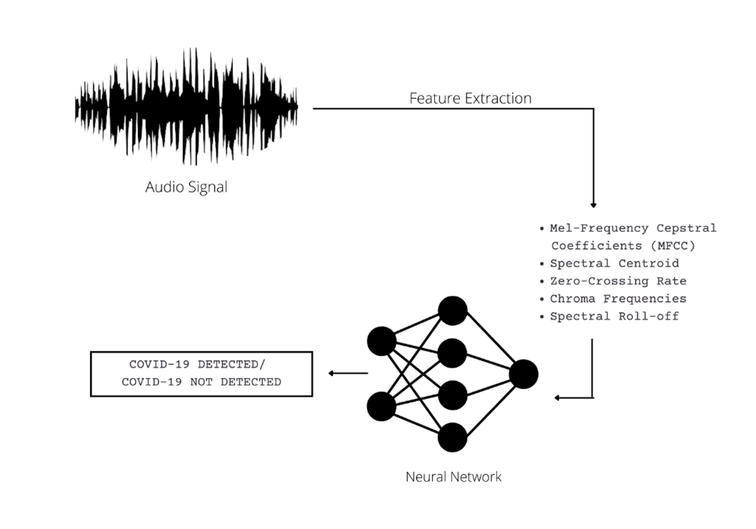
COVID-19 Detection System with Cough Audio Analysis

The following features will be extracted from the audio files (a brief explanation of each is given along with):

1. Mel-frequency cepstral coefficients (MFCC) (20 in number): · Mel-frequency cepstral coefficients (MFCCs) are coefficients that collectively make up an MFC. They are derived from a type of cepstral representation of the audio clip. The difference between the cepstrum and the Mel-frequency cepstrum is that in the latter, the frequency bands are equally spaced on the Mel scale, which approximates the human auditory system’s response more closely than the linearly-spaced frequency bands used in the normal spectrum. This frequency warping can allow for better representation of sound, for example, in audio compression.

2. Spectral Centroid: It measures the amplitude at the centre of the spectrum of the signal distribution over a window calculated from the Fourier-Transform frequency and amplitude information.

3. Zero-Crossing Rate: · The zero-crossing rate (ZCR) is the rate at which a signal transitions from positive to zero to negative or negative to zero to positive. Its value has been extensively used in speech recognition and music information retrieval for classifying percussive sounds.

4. Chroma Frequencies: Chroma features are a powerful representation of audio in which the entire spectrum is projected onto 12 bins representing the 12 different semitones (or chroma).

5. Spectral Roll-off: Spectral roll-off is the frequency below which a defined percentage of the total spectral energy lies.

All these features are characteristics of the audio and can be used to categorize the audio distinctively. Thus, we can conclude that the methodology we intend to adopt – converts the audio-classification problem into a numeric-data-classification problem.

Data Pre-Processing

In the pre-processing phase, we’ll extract the values of the abovementioned features from the audio files. This can be accomplished by using Python’s audio processing library Librosa. 

Installation:

Librosa can be installed using pip as follows:

pip install librosa

The stepwise Python implementation of the feature extraction phase is given below:

1. Import Necessary Libraries

Following are the libraries we need to import.

import pandas 
import numpy 
import os
import pathlib
import csv
from sklearn.model_selection import train_test_split
from sklearn.preprocessing import LabelEncoder, StandardScaler

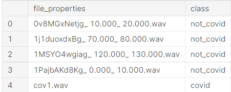
2. Load the Dataset

Now, we’ll load the dataset. Our dataset is a CSV file comprising the paths of the audio files and their respective labels.

The data looks as follows:

3. Making all the Header Fields for the Final Dataset (Optional)

In this step, we define the header files of the new dataset we will obtain post-feature extraction. This is an optional step.

header = 'filename chroma_stft rmse spectral_centroid spectral_bandwidth rolloff zero_crossing_rate'
for i in range(1, 21):
    header += f' mfcc{i}'
header += ' label'
header = header.split()

header

Output:

['filename',
 'chroma_stft',
 'rmse',
 'spectral_centroid',
 'spectral_bandwidth',
 'rolloff',
 'zero_crossing_rate',
 'mfcc1',
 'mfcc2',
 'mfcc3',
 'mfcc4',
 'mfcc5',
 'mfcc6',
 'mfcc7',
 'mfcc8',
 'mfcc9',
 'mfcc10',
 'mfcc11',
 'mfcc12',
 'mfcc13',
 'mfcc14',
 'mfcc15',
 'mfcc16',
 'mfcc17',
 'mfcc18',
 'mfcc19',
 'mfcc20',
 'label']

4. Feature Extraction 

This is the most crucial step of the pre-processing phase. Here, we convert our audio files into numeric data. As stated earlier, this is done using Librosa. Here we read each audio file, extract its features using Librosa’s in-built modules and store them in a new CSV file.

import librosa
file = open('data_new_extended.csv', 'w')
with file:
    writer = csv.writer(file)
    writer.writerow(header)
for i in range(tot_rows):
        source = train_csv['file_properties'][i]
        file_name = '../input/coughclassifier-trial/trial_covid/'+source
        y,sr = librosa.load(file_name, mono=True, duration=5)
        chroma_stft = librosa.feature.chroma_stft(y=y, sr=sr)
        rmse = librosa.feature.rms(y=y)
        spec_cent = librosa.feature.spectral_centroid(y=y, sr=sr)
        spec_bw = librosa.feature.spectral_bandwidth(y=y, sr=sr)
        rolloff = librosa.feature.spectral_rolloff(y=y, sr=sr)
        zcr = librosa.feature.zero_crossing_rate(y)
        mfcc = librosa.feature.mfcc(y=y, sr=sr)
        to_append = f'{source[:-3].replace(".", "")} {np.mean(chroma_stft)} {np.mean(rmse)} {np.mean(spec_cent)} {np.mean(spec_bw)} {np.mean(rolloff)} {np.mean(zcr)}'    
        for e in mfcc:
            to_append += f' {np.mean(e)}'
        
        file = open('data_new_extended.csv', 'a')
        with file:
            writer = csv.writer(file)
            writer.writerow(to_append.split())

Now, let’s load the newly formed dataset.

data1 = pd.read_csv('../input/coughclassifier-trial/data_new_extended.csv')
data1

 5. Pre-Processing the New Dataset for Model Training

After obtaining the data in numeric form, it is imperative to undergo pre-processing to deem fit for model training. The following steps encompass the pre-processing of numeric data:

– Dropping unnecessary columns:

# Dropping unneccesary columns
data1 = data1.drop(['filename'],axis=1)

– Label Encoding the output Labels:

labels = data1.iloc[:, -1]
encoder = LabelEncoder()
y = encoder.fit_transform(labels)

– Standard Scaling the Input Features:

scaler = StandardScaler()

X = scaler.fit_transform(np.array(data1.iloc[:, :-1], dtype = float))

– Splitting the data into Train and Test datasets:

X_train, X_test, y_train, y_test = train_test_split(X, y, test_size=0.2)

Model Building and Training

To classify the pre-processed audio data, one has many models and options available; however, determining the best model is the key. Since we had numerical data (obtained after pre-processing the audio signals), we will use an ANN (Artificial Neural Network) that will be trained on 80% of the data – the remaining 20% will be used for testing.

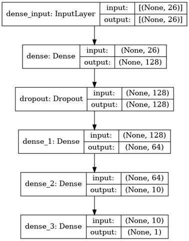
The following diagram depicts in great detail the architecture of the model that was employed to accomplish the classification:

 

The stepwise approach to model building and training is as follows:

1. Import Necessary Libraries

The following libraries need to be imported:

import tensorflow as tf
from tensorflow import keras
from keras import models
from keras import layers
from keras.layers import Dropout

2. Creating the Model

Firstly, we define a sequential model and then subsequently add layers to it – as per the architecture defined above. Please note that the architecture has been devised using hyperparameter tuning.

model = tf.keras.Sequential()
model.add(layers.Dense(128, activation='relu', input_shape=(X_train.shape[1],)))

model.add(Dropout(0.3, input_shape=(60,)))

model.add(layers.Dense(64, activation='relu'))

model.add(layers.Dense(10, activation='relu'))

model.add(layers.Dense(1, activation='sigmoid'))

Let us now look at the model summary:

model.summary()

Model: "sequential"
_________________________________________________________________
Layer (type)                 Output Shape              Param #   
=================================================================
dense (Dense)                (None, 128)               3456      
_________________________________________________________________
dropout (Dropout)            (None, 128)               0         
_________________________________________________________________
dense_1 (Dense)              (None, 64)                8256      
_________________________________________________________________
dense_2 (Dense)              (None, 10)                650       
_________________________________________________________________
dense_3 (Dense)              (None, 1)                 11        
=================================================================
Total params: 12,373
Trainable params: 12,373
Non-trainable params: 0
_________________________________________________________________

Since we are dealing with simplified numeric data, all the layers operate in a single dimension. The first layer is the input layer. Following this is the first dense layer with 128 neurons. To counter overfitting training data, the mode makes use of dropout regularization. For this, the third layer is a dropout layer. To ensure that the data is deciphered better, there are three more dense layers comprising 128, 64, and 10 neurons each.

Choice of activation functions: At the output layer, the binary classification task is accomplished using a sigmoid activation function. It is the most common choice in the case of binary classification. For all dense and dropout layers – the ReLU Activation function is used.

3. Model Compilation and Training 

We’ll compile the model as follows:

– Optimizer: Adam

– Loss Function: binary_crossentropy

– Metric: Accuracy

Furthermore, we will train the model for 15 epochs.

model.compile(optimizer='adam',loss='binary_crossentropy',metrics=['accuracy'])
model.fit(X_train, y_train, epochs=15)

Epoch 1/15
5/5 [==============================] - 1s 3ms/step - loss: 0.6509 - accuracy: 0.6397
Epoch 2/15
5/5 [==============================] - 0s 3ms/step - loss: 0.5321 - accuracy: 0.8529
Epoch 3/15
5/5 [==============================] - 0s 3ms/step - loss: 0.4392 - accuracy: 0.8897
Epoch 4/15
5/5 [==============================] - 0s 3ms/step - loss: 0.3640 - accuracy: 0.8897
Epoch 5/15
5/5 [==============================] - 0s 3ms/step - loss: 0.2974 - accuracy: 0.8897
Epoch 6/15
5/5 [==============================] - 0s 3ms/step - loss: 0.2606 - accuracy: 0.8897
Epoch 7/15
5/5 [==============================] - 0s 3ms/step - loss: 0.2450 - accuracy: 0.8897
Epoch 8/15
5/5 [==============================] - 0s 3ms/step - loss: 0.2168 - accuracy: 0.8897
Epoch 9/15
5/5 [==============================] - 0s 3ms/step - loss: 0.2085 - accuracy: 0.8897
Epoch 10/15
5/5 [==============================] - 0s 3ms/step - loss: 0.1767 - accuracy: 0.8897
Epoch 11/15
5/5 [==============================] - 0s 3ms/step - loss: 0.1537 - accuracy: 0.9265
Epoch 12/15
5/5 [==============================] - 0s 3ms/step - loss: 0.1255 - accuracy: 0.9559
Epoch 13/15
5/5 [==============================] - 0s 3ms/step - loss: 0.1294 - accuracy: 0.9632
Epoch 14/15
5/5 [==============================] - 0s 3ms/step - loss: 0.1129 - accuracy: 0.9632
Epoch 15/15
5/5 [==============================] - 0s 3ms/step - loss: 0.0973 - accuracy: 0.9853

Thus, the training accuracy is 98%  

4. Testing the Model 

Now, we test the model on the testing dataset.

test_loss, test_acc = model.evaluate(X_test,y_test)

2/2 [==============================] - 0s 6ms/step - loss: 0.1306 - accuracy: 0.9412

Thus, the testing accuracy is 94%

Link to Kaggle Notebook: The Kaggle notebook wherein the project has been implemented can be found here.

Conclusion 

Based on the performance of our technology on both the training/validation and prospective data sets, we conclude that it is indeed possible to accurately and objectively diagnose COVID-19 cough sounds alone using cough sound analysis. It is possible to augment cough-based features with simple symptoms observable by parents targeting further performance improvement. Though the accuracy level is quite high and acceptable – it must be noted that the study proposes the model only for preliminary diagnosis of COVID-19 and that the results must be taken as indicative.

Key Takeaways:

After having gone through this article we:

– Have gained an understanding of audio processing using Librosa 

– Have devised a simple way to diagnose COVID-19 with cough audio analysis.

– Have built an ANN model that classifies audios of patients into COVID-positive/COVID-negative categories after a cough audio analysis.

Though the results might vary on datasets, the model lays the groundwork for the imperative task of COVID-19 cough classification using MFCC feature extraction and ANN modelling. This has an immense future scope as it can form the basis for classification and, thus, diagnosis of any respiratory ailment with characteristics of cough audio which is usually the case.

Furthermore, the presented approach can be integrated into a mobile application to make this entire study a wholesome product.