Comparison of the RMS Energy and the Amplitude Envelope
This article was published as a part of the Data Science Blogathon.
Introduction
Have you ever wondered what an audio’s Amplitude Envelope and RMS energy are? And, if you had to choose, which of these do you believe would be most resilient to outliers? If these questions pique your interest, then this article is for you!
In this article, we’ll visualize and examine the RMS Energy and the Amplitude Envelope of different music genre tracks, including classical, blues, reggae, rock, and jazz, using the librosa library, and then subsequently uncover which of these features are more robust to the outliers. Valerio Valerdo’s work served as inspiration for this article. I strongly advise you to visit his Youtube channel to see his remarkable work in the field of audio ML/DL.
Tools
- Python,
- Librosa,
- Audio samples from the GTZAN dataset (each sample is 30 seconds long)
What does RMS Energy Mean?
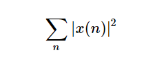
RMS Energy of the audio signal: The overall magnitude of a signal corresponds to its energy. For audio signals, this generally equates to how loud the signal is. The signal’s energy is calculated as follows:
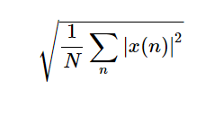
RMS is a useful method of computing the average of variables across time. When dealing with audio, the signal value (amplitude) is squared, averaged over time, and then the square root of the result is determined. The mathematical definition of a signal’s root-mean-square energy (RMSE) is:
What does the Amplitude Envelope of the Audio Signal Mean?
Amplitude Envelope: The amplitude envelope is a time-domain audio characteristic extracted from the raw audio waveform that refers to fluctuations in a sound’s amplitude over time and is an important quality because it affects our auditory impression of timbre. This is a crucial sound feature because it allows us to recognize and discriminate sounds quickly. The signal’s Amplitude Envelope, which offers a rough estimate of loudness, is made up of the maximum amplitude values across all samples in each frame. This property has been widely used for music genre classification and onset detection. However, because it is more sensitive to outliers than the RMS energy audio function, it is frequently less preferred.
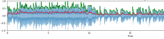
Waveplots depicting the RMS energy (shown in red) and the amplitude envelope (shown in green)
Now, without further ado, let’s have a look at the RMS energy of the various music genre audio signals, and alongside, let’s compare them to their corresponding amplitude envelopes. [For more details on Amplitude Envelope, please take a look at my previous post].
The following is a step-by-step guide to visualizing and comparing the Amplitude envelope and RMS energy of different music genre tracks.
Step 1: Install and Import all of the Required Dependencies
First, we will import all of the required packages and specify the path of the audio files, after which we will load it with librosa.
!pip install librosa
import matplotlib.pyplot as plt
import numpy as np
import librosa
import librosa.display
import IPython.display as ipd
%matplotlib inline
Step 2: Load the Audio Files
#Specifying the path to audio files
classical_music_file = "/content/drive/MyDrive/trytheseaudios/classical.00000.wav"
blues_music_file = "/content/drive/MyDrive/trytheseaudios/blues.00000.wav"
reggae_music_file = "/content/drive/MyDrive/trytheseaudios/reggae.00000.wav"
rock_music_file = "/content/drive/MyDrive/trytheseaudios/rock.00000.wav"
jazz_music_file = "/content/drive/MyDrive/trytheseaudios/jazz.00000.wav"
The audio files will then be loaded as a floating-point time series.
# load audio files with librosa
classical, sr = librosa.load(classical_music_file)
blues, _ = librosa.load(blues_music_file)
reggae, _ = librosa.load(reggae_music_file)
rock, _ = librosa.load(rock_music_file)
jazz, _ = librosa.load(jazz_music_file)
Step 3: Compute the RMS energy of Each Signal using Librosa
Now we will compute the RMS energy of each signal using Librosa.
FRAME_SIZE = 1024
HOP_LENGTH = 512
rms_classical = librosa.feature.rms(classical, frame_length=FRAME_SIZE, hop_length=HOP_LENGTH)[0]
rms_blues = librosa.feature.rms(blues, frame_length=FRAME_SIZE, hop_length=HOP_LENGTH)[0]
rms_reggae = librosa.feature.rms(reggae, frame_length=FRAME_SIZE, hop_length=HOP_LENGTH)[0]
rms_rock = librosa.feature.rms(rock, frame_length=FRAME_SIZE, hop_length=HOP_LENGTH)[0]
rms_jazz = librosa.feature.rms(jazz, frame_length=FRAME_SIZE, hop_length=HOP_LENGTH)[0]
Following that, we will define a function for computing the amplitude envelope for different music genre songs.
Step 4: Write a Block of Code for Calculating the Amplitude Envelope
#Function for calculating the amplitude envelope
def amplitude_envelope(signal, frame_size, hop_length):
  return np.array([max(signal[i:i+frame_size]) for i in range(0, signal.size, hop_length)])
Step 5: Compute the Amplitude Envelope for Individual Genre Track
#Amplitude Envelope for individual genre
ae_classical = amplitude_envelope(classical, FRAME_SIZE, HOP_LENGTH)
ae_blues = amplitude_envelope(blues, FRAME_SIZE, HOP_LENGTH)
ae_reggae = amplitude_envelope(reggae, FRAME_SIZE, HOP_LENGTH)
ae_rock = amplitude_envelope(rock, FRAME_SIZE, HOP_LENGTH)
ae_jazz = amplitude_envelope(jazz,FRAME_SIZE, HOP_LENGTH)
Finally, let us visualize and compare RMS energy and magnitude envelope charts in order to derive some conclusions.
Step 6: Visualize and Compare the RMS Energy and the Amplitude Envelope of Different Music Genre Tracks
#Visualise RMSE + waveform
frames = range(len(rms_classical))
t = librosa.frames_to_time(frames, hop_length=HOP_LENGTH)
# rms energy is graphed in red
plt.figure(figsize=(20, 20))
ax = plt.subplot(5, 1, 1)
librosa.display.waveplot(classical, alpha=0.5)
plt.plot(t, rms_classical, color="r")
plt.plot(t, ae_classical, color="g")
plt.ylim((-1, 1))
plt.title("Classical Music Genre song")
plt.subplot(5, 1, 2)
librosa.display.waveplot(blues, alpha=0.5)
plt.plot(t, rms_blues, color="r")
plt.plot(t, ae_blues, color="g")
plt.ylim((-1, 1))
plt.title("Blues Music Genre song")
plt.subplot(5, 1, 3)
librosa.display.waveplot(reggae, alpha=0.5)
plt.plot(t, rms_reggae, color="r")
plt.plot(t, ae_reggae, color="g")
plt.ylim((-1, 1))
plt.title("Reggae Music Genre Song")
plt.subplot(5, 1, 4)
librosa.display.waveplot(rock, alpha=0.5)
plt.plot(t, rms_rock, color="r")
plt.plot(t, ae_rock, color="g")
plt.ylim((-1, 1))
plt.title("Rock Music Genre song")
plt.subplot(5, 1, 5)
librosa.display.waveplot(jazz, alpha=0.5)
plt.plot(t, rms_jazz, color="r")
plt.plot(t, ae_jazz, color="g")
plt.ylim((-1, 1))
plt.title("Jazz Music Genre song")
plt.subplots_adjust(hspace = 0.75)
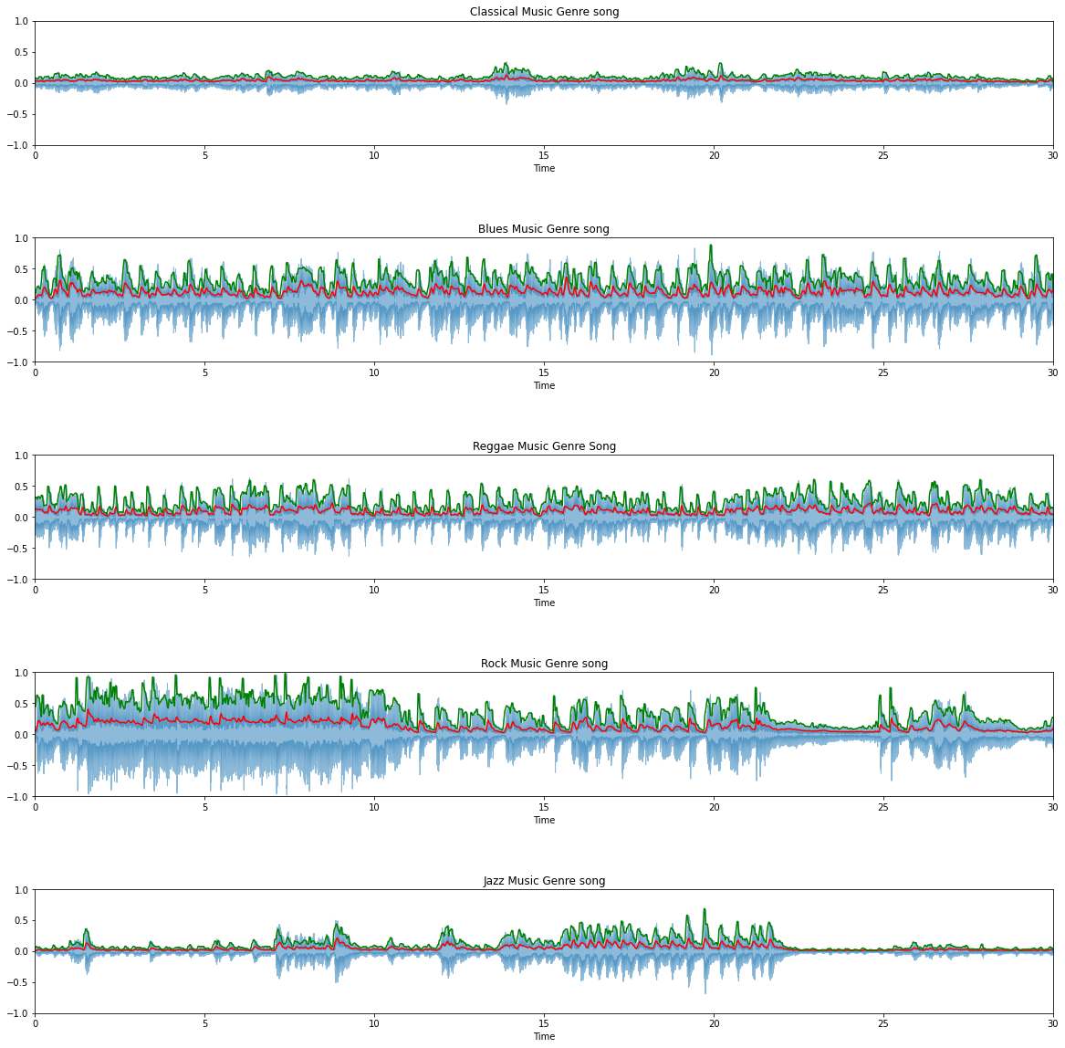
Waveplots depicting the amplitude envelope (shown in green) and the RMS energy (shown in red) of different music genres
Visual inspection reveals that the amplitude envelope (shown in green) contains many spikes and follows the waveform’s outer contour, making it more susceptible to outliers. However, because we are considering the RMS energy of all samples in a frame, the RMS energy plot (shown in red) is significantly smoother. Furthermore, we can see that the amplitude envelope of Blues, Rock, Reggae, and Jazz music genre songs has a lot more artefacts than Classical music genre songs due to the low variability.
Conclusion
Upon visual inspection, we can see that the amplitude envelope (shown in green) contains a lot of spikes and follows along the outer contour of the waveform, making it more susceptible to outliers. On the other hand, the plot (shown in red) is much smoother as we are considering the RMS energy of all samples in a frame. Furthermore, we can see that the amplitude envelope of Blues, Rock, Reggae, and Jazz music genre songs has a lot more artefacts than Classical music genre songs due to the low variability. However, we cannot generalize this to the entire music genre based on these cases. But, indeed, the above wave-plot analysis might provide us with a quick overview, sort of intuition about different music genres.
To summarize, the key takeaways from this article were:
- We learned what the RMS Energy and the Amplitude Envelope of audio are.
- We used Librosa to visualize and compare the RMS Energy and the Amplitude Envelope of different music genre tracks.
- We also learned about the drawbacks of Amplitude Envelope over RMS Energy.
Link to GitHub Repo – Click here!
Thanks for reading. If you have any questions or concerns, please leave them in the comments section below. Happy Learning!
The media shown in this article is not owned by Analytics Vidhya and is used at the Author’s discretion.


