Machine Learning Models Comparative Analysis

This article was published as a part of the Data Science Blogathon.

Introduction

Machine learning uses a mathematical and statistical way to learn. Predicting in machine learning can be done with many methods and models. There are several uses for this, like OCR, spam detection, etc.

Source: fs.ac.in/blog/

In this article, we will use the Book-My-Show dataset and apply three machine learning models to analyze which model is suitable for this dataset.

Problem Affirmation

To tackle the Book-My-Show problem, we will use Logistic Regression, KNeighbors, and XGB for the prediction. We will draw a conclusion about which model works best. 

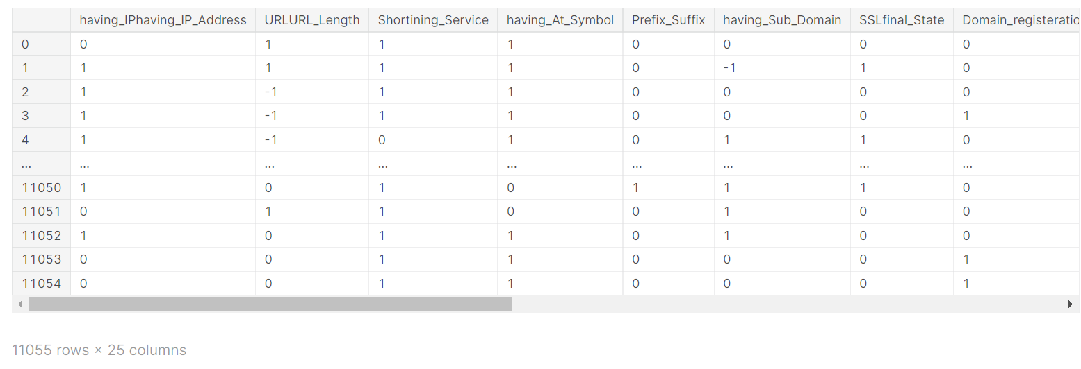
About Dataset of Book-My-Show

The 11k sample corresponds to an 11k URL in the input dataset. Each sample has a different description of the URL with different values. The URL may be a legitimate or phishing link if it is in the range of -1 (suspicious),0 (phishing), or 1 (legitimate).

Implementation

The practical is implemented in Kaggle. You can access the dataset and notebook through the following links. The book-my-show notebook link is on my kaggle.com account.

Dataset Link: https://www.kaggle.com/datasets/shibumohapatra/book-my-show 

Notebook Link: https://www.kaggle.com/code/shibumohapatra/logistics-regression-kneighbors-xgb

Modules and Library Info

import numpy as np
import pandas as ad
import matplotlib.pyplot as plt
%matplotlib inline
import seaborn as sns
from sklearn.model_selection import train_test_split,cross_val_score
from sklearn.metrics import accuracy_score,confusion_matrix,classification_report
from sklearn.linear_model import LogisticRegression
from sklearn.neighbors import KNeighborsClassifier
from xgboost import XGBClassifier,cv
from sklearn.metrics import roc_curve, auc
from sklearn.model_selection import KFold
from sklearn.model_selection import cross_val_score, LeaveOneOut
from sklearn.model_selection import GridSearchCV, StratifiedKFold

Exploratory Data Analysis (EDA)

We need to explore the data using heat maps and histograms. The number of samples in the data and unique elements in all the features will be determined. We must check if there is a null value in any of the columns.

df_data = df_data.drop('index',1)

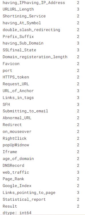
df_data.nunique()

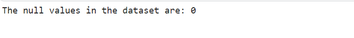
#check for NULL value in the dataset

print("The null values in the dataset are:",df_data.isnull().sum().sum())

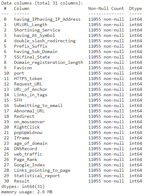
# NULL value check
df_data.info()

# Duplicate check
df1 = df_data.T
print("The duplicate values in dataset is:",df1.duplicated().sum())

Plot histogram for data exploration

df_data.hist(bins=50, figsize=(20,15))
plt.show()

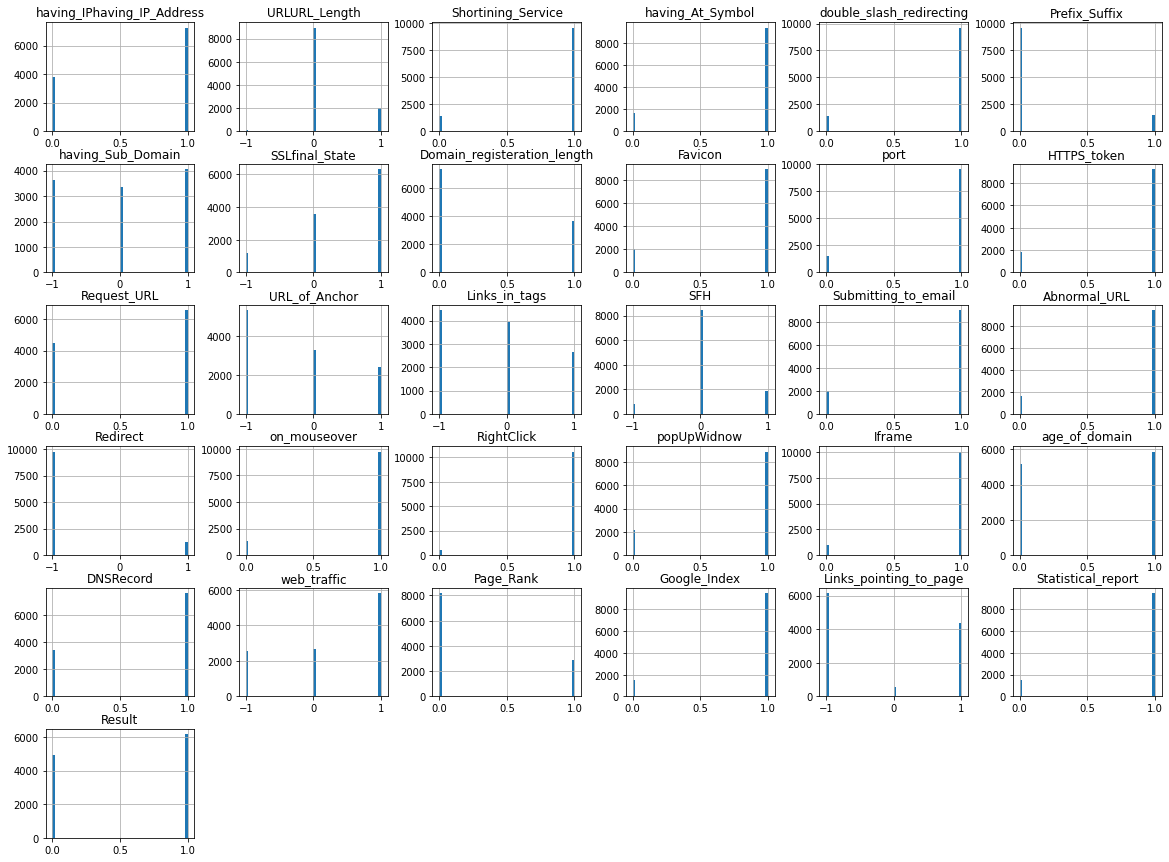
The distribution of the data is shown in the above histogram. -1, 0, and 1 are the values.

pd.value_counts(df_data['Result']).plot.bar()

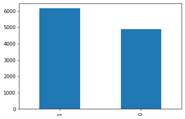
The distribution of Legitimate (1) URLs and Phishing (0) URLs is shown in the above graph.

Correlated Features and Feature Selection

We need to find out if there are any correlated features in the data and remove the feature which could be correlated with a threshold.

#correlation map
f,ax=plt.subplots(figsize=(18,18))
sns.heatmap(df_data.corr(),annot=True, linewidths=.5, fmt='.1f',ax=ax)

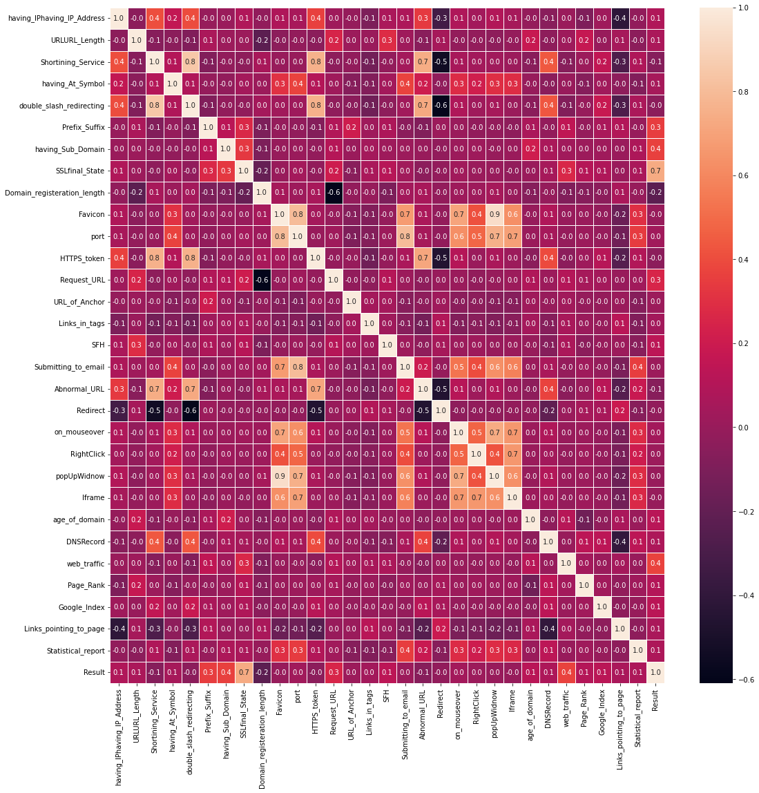
The above heatmap output “popUpWindow” and “Favicon” have a strong correlation of 0.9. It suggests data redundancy. So, one of the columns must be deleted.

There is a correlation between the heatmap output “popUpWindow” and “Favicon”. There are 9. It suggests there is more than one data source. One of the columns needs to be deleted. We need to find highly correlated independent variables and remove the columns. The threshold values were set at 0.75. The columns that have correlation values of more than 0. 75 will be removed.

cor_matrix = df_data.corr().abs()
upper_tri=cor_matrix.where(np.triu(np.ones(cor_matrix.shape),k=1).astype(np.bool))

# threshold greater than 0.75
to_drop = [column for column in upper_tri.columns if any(upper_tri[column] > 0.75)]
print(to_drop)

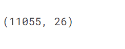
#drop the columns which are highly correlated
df_data.drop(to_drop,axis=1,inplace=True)
df_data.shape

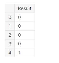
X=df_data.drop(columns='Result')
X

Y=df_data['Result']
Y= pd.DataFrame(Y)
Y.head()

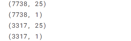
Here, we will split the data into train and test sets.

# split train - test to 70-30
train_X,test_X,train_Y,test_Y = train_test_split(X,Y,test_size=0.3, random_state=9)

print(train_X.shape)
print(train_Y.shape)
print(test_X.shape)
print(test_Y.shape)

Classification Model

A classification model can be built if we clearly understand the data. A classification model is first developed to identify malicious URLs.

#model build for different binary classification and show confusion matrix
def build_model(model_name,train_X, train_Y, test_X, test_Y):
   if model_name == 'LogisticRegression':
       model=LogisticRegression()
   elif model_name =='KNeighborsClassifier':
       model = KNeighborsClassifier(n_neighbors=4)
   elif model_name == 'XGBClassifier':
       model = XGBClassifier(objective='binary:logistic',eval_metric='auc')
   else:
       print('not a valid model name')
   model=model.fit(train_X,train_Y)
   pred_prob=model.predict_proba(test_X)
   fpr, tpr, thresh = roc_curve(test_Y, pred_prob[:,1], pos_label=1)
   model_predict= model.predict(test_X)
   acc=accuracy_score(model_predict,test_Y)
   print("Accuracy: ",acc)
   # Classification report
   print("Classification Report: ")
   print(classification_report(model_predict,test_Y))
   #print("Confusion Matrix for", model_name)
   con =  confusion_matrix(model_predict,test_Y)
   sns.heatmap(con,annot=True, fmt ='.2f')
   plt.suptitle('Confusion Matrix for '+model_name, x=0.44, y=1.0, ha='center', fontsize=25)
   plt.xlabel('Predict Values', fontsize =25)
   plt.ylabel('Test Values', fontsize =25)
   plt.show()
   return model, acc, fpr, tpr, thresh

We will use a heatmap to see the confusion matrix of each model and its performance once we have built all the models.

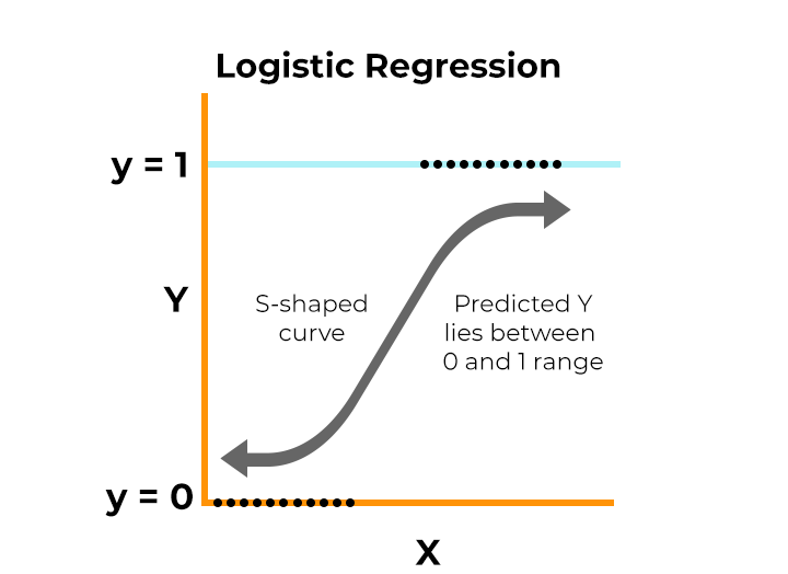
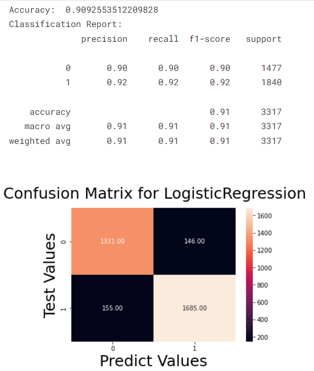
Model 1 – Logistic Regression

Logistic Regression is a supervised method. Logistic regression is used to calculate or predict events. There are two conditions: yes or no. A classic example is if a person is sick with a cold or not. Either the patient is infectious or they are not; that is the outcome. Logistic Regression has three types and one. A binomial has two outcomes, 0 or 1, which can be either win or lose. 2. There are more than two outcomes for multinomial. The categories of target variables, like test scores, have been ordered; the scores are 0,1, 2, and so on.

Source: Logistic Regression

# Model 1 - LogisticRegression
lg_model,acc1, fpr1, tpr1, thresh1 = build_model('LogisticRegression',train_X, train_Y, test_X, test_Y.values.ravel())

Source: Logistic Regression

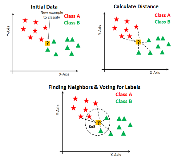
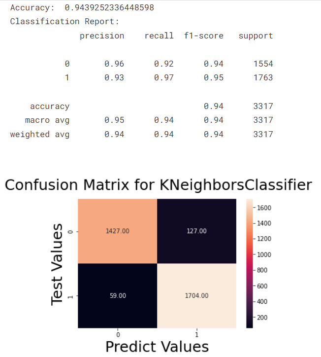
Model 2 – KNeighbors Classifier

This is a supervised method usually used for classification and regression problems. It is used for resampling. The new data points predict the class or continuous value. KNeighbors is a lazy machine-learning model.

 

Source: KNeighbors

# Model 2 - KNeighborsClassifier
knn_model,acc2, fpr2, tpr2, thresh2 = build_model('KNeighborsClassifier',train_X, train_Y, test_X, test_Y.values.ravel())

Source: KNeighbors

Model 3 – XGB Classifier

It is a form of machine learning that uses an ascendable and distributed decision tree. XGB provides a parallel tree boosting. The boosting technique is used in XGB to attempt to build a strong classifier.

# Model 3 - XGBClassifier
xgb_model, acc3, fpr3, tpr3, thresh3 = build_model('XGBClassifier',train_X, train_Y, test_X, test_Y.values.ravel())

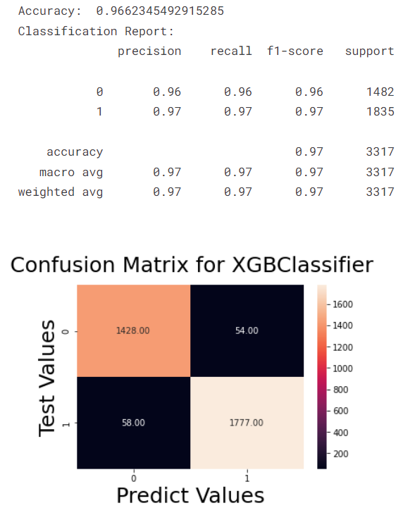
The above confusion matrix shows that the XGB classification has the highest accuracy.

We need to plot the ROC curve to show the diagnostic ability of this classifier.

# roc curve for tpr = fpr
random_probs = [0 for i in range(len(test_Y))]
p_fpr, p_tpr, _ = roc_curve(test_Y, random_probs, pos_label=1)

Plotting ROC curve

plt.style.use('seaborn')
# plot roc curves
plt.plot(fpr1, tpr1, linestyle='--',color='orange', label='Logistic Regression')
plt.plot(fpr2, tpr2, linestyle='--',color='green', label='KNN')
plt.plot(fpr3, tpr3, linestyle='--',color='red', label='XGBClassifier')
plt.plot(p_fpr, p_tpr, linestyle='--', color='blue')
# title
plt.title('ROC curve')
# x label
plt.xlabel('False Positive Rate')
# y label
plt.ylabel('True Positive rate')
plt.legend(loc='best')
plt.savefig('ROC',dpi=300)
plt.show()

 

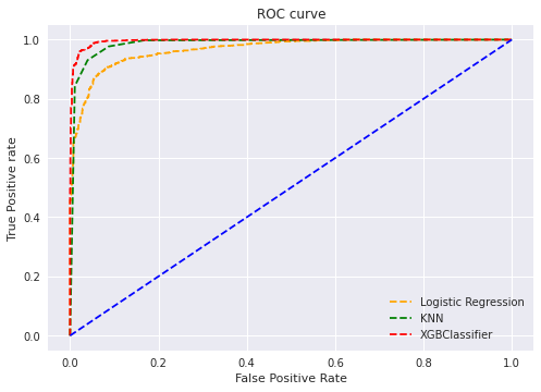
Shown by the ROC plot is XGBClassifier Compared to other models, the (TPR) True Positive Rate is higher.

We need to use the K-Fold cross-validation to verify the accuracy of the data we plot. We will use the GridSearchCV to find the best parameters of different models and the StratifiedKFold cross-validation techniques to find data accuracy.

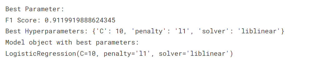
Liblinear and newton-CG solver and l1, l2 penalty for Logistic Regression Model evaluation

For Logistic Regression, we drew 91% accuracy in 4 StratifiedKFold folds.

import warnings
warnings.filterwarnings("ignore")
# Create the parameter grid based on the results of random search
param_grid = {
   'solver':['liblinear','newton-cg'],
   'C': [0.01,0.1,1,10,100],
   'penalty': ["l1","l2"]
}
# Instantiate the grid search model
grid_search = GridSearchCV(estimator = LogisticRegression() , param_grid = param_grid,
cv = StratifiedKFold(4), n_jobs = -1, verbose = 1, scoring = 'accuracy' )
grid_search.fit(train_X,train_Y.values.ravel())

print('Best Parameter:')
print('F1 Score:', grid_search.best_score_)
print('Best Hyperparameters:', grid_search.best_params_)
print('Model object with best parameters:')
print(grid_search.best_estimator_)

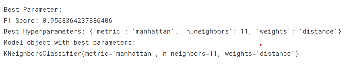
GridSearchCV technique for KNeighborsClassifier Model evaluation

For KNeighbors classifier, we acquired 95% accuracy in 3 GridSearchCV folds.

grid_params = {
   'n_neighbors':[3,4,11,19],
   'weights':['uniform','distance'],
   'metric':['euclidean','manhattan']
}
gs= GridSearchCV(
KNeighborsClassifier(),
grid_params,
verbose=1,
cv=3,
n_jobs=-1
)
gs_results = gs.fit(train_X,train_Y.values.ravel())

print('Best Parameter:')
print('F1 Score:', gs_results.best_score_)
print('Best Hyperparameters:', gs_results.best_params_)
print('Model object with best parameters:')
print(gs_results.best_estimator_)

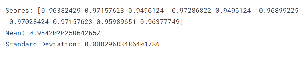
KFold cross-validation technique for XGBClassifier model

For XGB Classifier, we acquired 96% accuracy in 10 folds.

xgb_cv = XGBClassifier(n_estimators=100,objective='binary:logistic',eval_metric='auc')
scores = cross_val_score(xgb_cv, train_X, train_Y.values.ravel(), cv=10, scoring = "accuracy")
print("Scores:", scores)
print("Mean:", scores.mean())
print("Standard Deviation:", scores.std())

Model Comparison

The final output of the model will give maximum accuracy on the validation dataset with selected attributes. The output of the below code shows that XGBoost is the winner and is an appropriate model for Ads URLs analysis.

results=pd.DataFrame({'Model':['LogisticRegression','KNeighbors','XGB'],
                    'Accuracy Score':[acc1,acc2,acc3]})
result_df=results.sort_values(by='Accuracy Score', ascending=False)
result_df=result_df.set_index('Model')
result_df

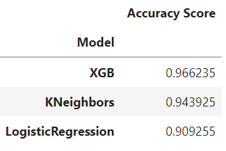
Comparison Table

Conclusion

The above implementation helps us to identify which machine learning model is suited for the Ads URL. The basic structure of the data was analyzed with Exploratory Data Analysis. We could understand the dataset’s features with the help of histograms and heat maps. We gathered the accuracy metrics of each model and made a comparison table that shows the overall accuracies of each model. The XGBoost model is the winner of the three machine learning models with an accuracy of 96 percent. The KNeighbors got a score of 94 percent. Logistic Regression got 90 percent.

Key Takeaways –

• The KNeighbors model was slower than the other two because it only outputs the labels.
• Logistic Regression was not flexible enough to capture more complex relationships.
• The other two models were slower than the XGB model.
• XGB has the ability to deal with both continuous and categorical data.
• The XGBoost model is appropriate for the Book-My-Show problem because of the above implementation.

Hopefully, the above implementation will help with selecting a machine-learning model.

The media shown in this article is not owned by Analytics Vidhya and is used at the Author’s discretion.