RetinaNet : Advanced Computer Vision
This article was published as a part of the Data Science Blogathon.
Introduction
RetinaNet is a single-stage object detection model that uses a focal loss function to deal with class imbalance during training. Focal loss applies a modulation term to the cross-entropy loss to focus learning on hard negative examples. Retina-Net is a single unified network consisting of a major back network and two task-specific subnetworks. The backbone is accountable for computing a convolutional characteristic map over the whole input image and is an off-the-self convolutional network. The first subnet performs convolutional object classification on the backbone output; the second subnet performs convolutional bounds regression. These two subnets have a simple design that the authors propose specifically for one-step dense detection.
FAIR released two papers in 2017 and 2018 on their state-of-the-art object detection frameworks. We’ll see how the various layers come together to form a robust object detection pipeline. As usual, I will use a mathematical approach to explain everything. We will briefly discuss the following two articles.
Anchor boxes
Anchor boxes were first introduced in the Faster RCNN paper and later became a common feature in all subsequent papers, such as yolov2, SSD, and RetinaNet. Previously, selective search and bounding boxes were used to generate region designs of different sizes and shapes depending on the objects in the image. With standard convolutions, generating region designs of different shapes is highly impossible, so anchor boxes help us.
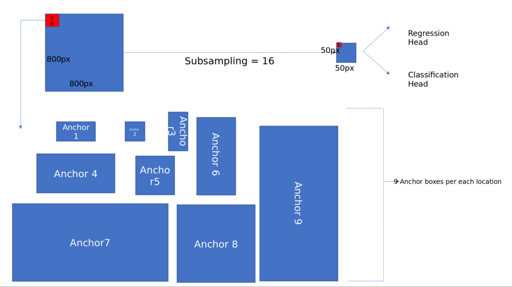
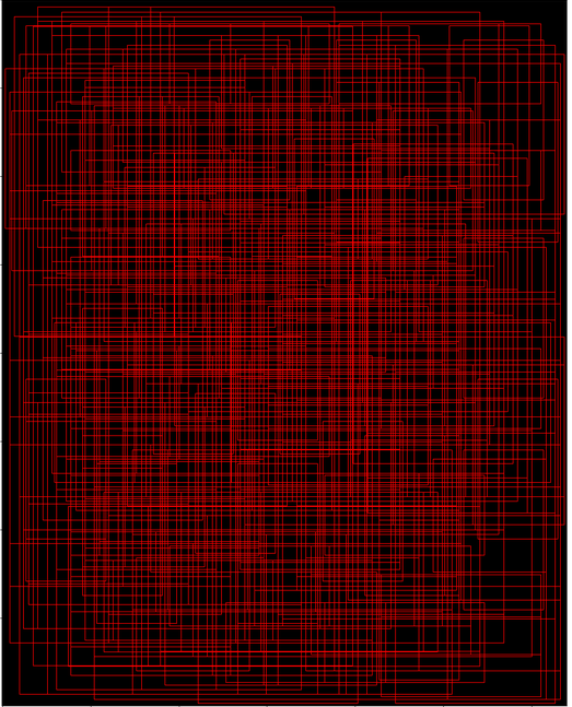
The diagram below helps in showing the valid anchor fields in the image,
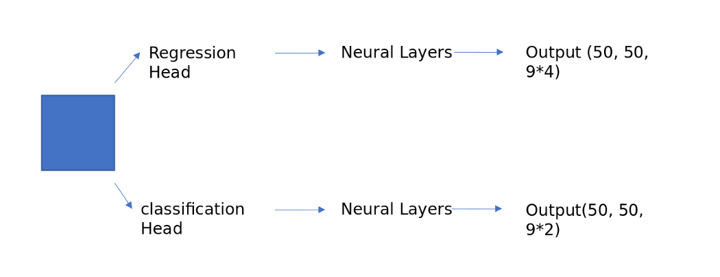
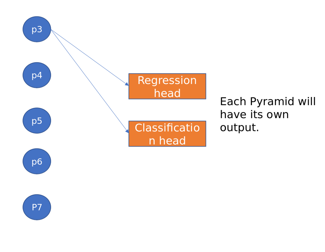
How does RPN work?
Classification head: Similar to the regression head, this will predict the probability of the presence or absence of an object at each location for each anchor foot. This is described in a NumPy array as np. array(2500, 9)
Problems with RPN
Working on Feature Pyramid Networks
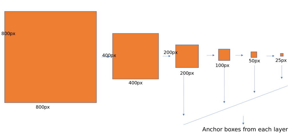
In RPN, we created anchor boxes using only the top-level feature map. Although convnets are robust to scale variation, all of the best entries in ImageNet or COCO used multiscale testing on selected image pyramids. Imagine taking an 800 * 800 image and detecting bounding boxes on it. Now, if you use image pyramids, we need to take images in different sizes like 256*256, 300*300, 500*500 and 800*800, etc., calculate feature maps for each of these images and then apply non-maximal suppression to all of these detected positive anchor boxes. This is a costly operation, and the derivation times increase.
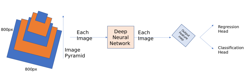
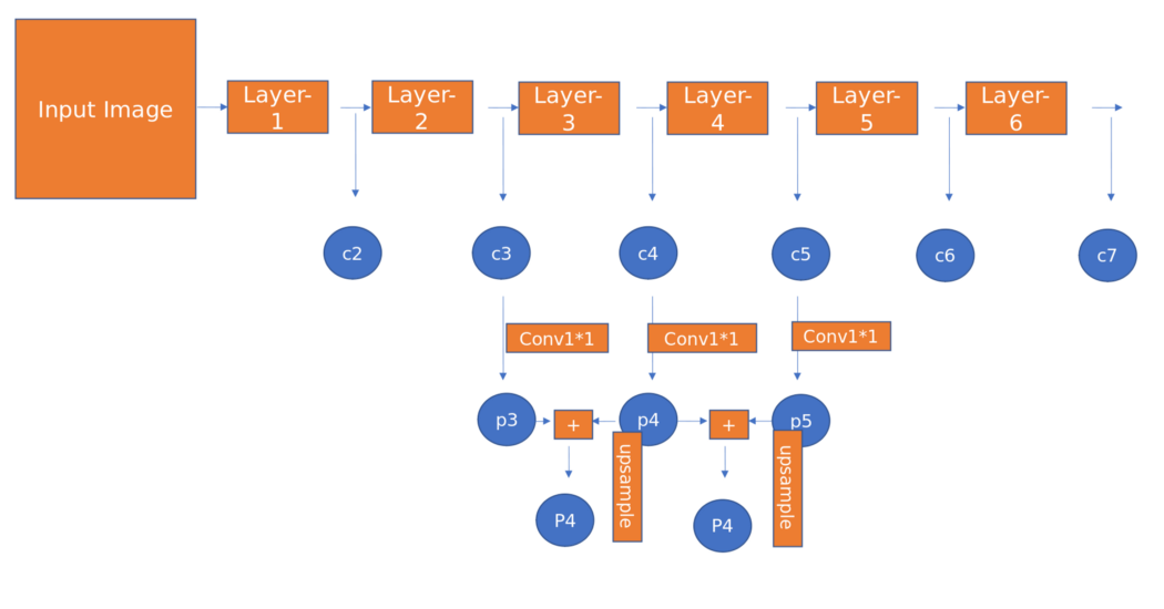
The authors of this paper observed that the deep convnet computes the feature hierarchy layer by layer. The feature hierarchy has its own multi-level, pyramidal shape with subsampling layers. For example, take the Resnet architecture, and instead of just using the final feature map as shown in the RPN network, take the feature maps before each pooling (subsampling) layer. Perform the same operations as for RPN on each feature map and combine them using non-maximal suppression. This is a rough way of building element pyramid networks. But there is one problem with this approach. Different depths cause large semantic gaps. High-resolution maps (earlier layers) have low-level features that impair their representational capacity for object detection.
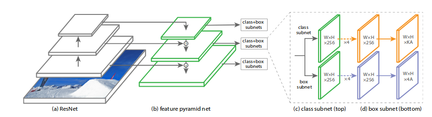
The author’s goal is to naturally take advantage of the pyramidal shape of Convnet’s feature hierarchy and, at the same time, create a feature pyramid that has strong semantics at all scales. To achieve this, the authors opted for an architecture that combines semantically powerful low-resolution features and semantically strong high-resolution features through a top-down path and side-connection, as shown in the figure below.
Some Important points while designing anchor boxes:
- Since the pyramids have different scales, there is no need to have anchors with multiple scales at a particular level. We define anchors as sizes [32, 54, 128, 256, 512] on P3, P4, P5, P6, and P7. We use anchors with multiple aspect ratios [1:1, 1:2, 2:1]. so there will be 15 anchors above the pyramid at each location.
- All anchor boxes outside the dimensions of the image were ignored.
- Positive if the given anchor box has the highest IoU with the ground truth box or if the IoU is more than 0.7. negative if IoU is minimum to 0.3.
- The weights of the basic truth boxes are not used to assign them to the pyramid levels. Instead, the ground truth boxes are associated with anchors assigned to the pyramids’ levels. I had two confusions here because we need to assign ground truth boxes to each level separately or calculate all anchor boxes and then assign the label to the anchor box with which it has a maximum IoU or IoU greater than 0.7. In the end, I chose the second option of assigning labels.
Implementation details on coco:
Focal Loss
CE loss:
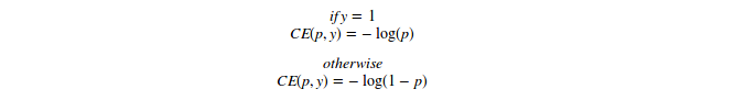
Binary cross entropy loss
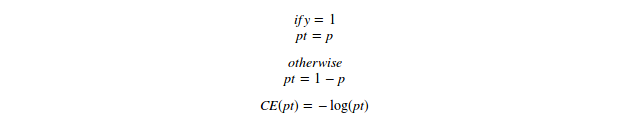
Binary cross entropy loss
For high-class imbalance, we add a weight parameter. it is usually the inverse class frequency or a hyperparameter set by cross-validation. Here we will call it alpha called balancing param.

Balancing param in Focal loss
As noted in the article, easily classifiable negatives make up most of the loss and dominate the gradient. Meanwhile, alpha balances the necessity of positive/negative examples. It does not differentiate between easy/hard examples. So the authors reshaped the cross entropy function and came up with the focal loss, as shown below.
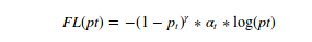
Focal loss equation
Here gamma is called focus param, and alpha is called equalization param.
Case 1: Simple, easy, correctly classified example
Case-2: misclassified example
Case-3: Very easily classified example
Important points to note
- When training object detection, the focal loss is applied to all ~100k anchors in each sampled image.
- The total image focal loss is calculated as the sum of the focal loss overall ~100k anchors, normalized by the number of anchors assigned to the base box.
- Gamma =2 and alpha =0.25 works best, and in general, alpha should decrease slightly as gamma increases.
RetinaNet for Object Detection
RetinaNet
RetinaNet Training
- Network initialization is very important. The authors assumed a prior probability of 0.01 for all anchor boxes and assigned that bias to the last Conv. Classification subnet layers. I overlooked this when implementing the network. The loss function will blow up if you don’t take care of it. The intuition behind attaching this prior probability is that the foreground (All positive anchor boxes) to background objects (All negative anchor boxes) in the image is 1000/100000 = 0.01.
- A weight drop of 0.0001 and a momentum of 0.9 with an initial learning rate of 0.01 is used for the first 60k iterations. The learning rate decreases by 10 after 60,000 iterations and 80,000 iterations.
- Achieved mAP 40.8 using ResNeXt-101-FPN backend on MS-coco dataset
Inference on RetinaNet
- To increase speed in RetinaNet, decode the box predictions from a maximum of 1000 top-scoring predictions to the FPN level after thresholding the detector confidence at 0.05.
- The best predictions from all levels are combined, and non-maximum suppression with a threshold of 0.5 is applied to arrive at the final decisions.
Conclusion
- RetinaNet is one of the best single-stage object detection models that work well with dense and small objects. For this reason, it has become a popular object detection model for aerial and satellite imagery use.
- RetinaNet was created by making two improvements over existing single-stage object detection models – Feature Pyramid Networks (FPN) [1] and Focal Loss [2].
- Case-1: 0.1/0.00026 = 384 times smaller number
- Case-2: 2.3/0.4667 = 5 times smaller number
- Case-3: 0.01/0.00000025 = 40,000 times smaller number.
If you want to learn “How one can establish a Face Mask Detector using RetinaNet Model,” please visit Article1 and Article2.
The media shown in this article is not owned by Analytics Vidhya and is used at the Author’s discretion.


Hi there, I read through your article, and it is very good and understandable. May I know how the two sub-networks that you mentioned that do not share the parameters do the back-propagation? Is it like classification loss does its own back-propagation and regression loss does its own back-propagation too, then they get their respective gradients, or do they sum up the total loss and then do the back-propagation? But if they use the total loss, there are two sub-networks; how can they get one gradient and use it for two sub-networks? Thank you very much, and hopefully I can get your reply soon.