Lightning fast CPU-based image captioning pipelines with Deep Learning and Ray
Jennifer Davis2022-06-14 | 14 min read
Translation between Skeletal formulae and InChI labels is a challenging image captioning problem, especially when it involves large amounts of noisy data. In this blog post we share our experience from the BMS molecular translation challenge and show that CPU-based distributed learning can significantly shorten model training times.
Background
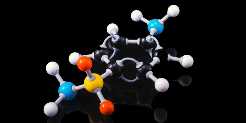
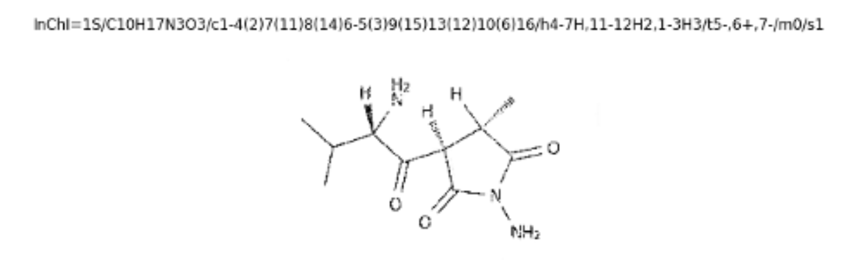
During 2000-2004, the International Union of Pure and Applied Chemistry (IUPAC) developed the InChI labeling system - a textual identifier for chemical substances, designed to provide a standard way to encode molecular information. InChI labels are essentially long strings of letters and symbols, created to enable the identification of chemicals and facilitate searches for them in databases and on the web. Having in mind that the InChI standard was officially released in 2005, it is understandable that predating chemical literature issues other means to describe chemical substances. The most common approach adopted in legacy documents is a pure graphical expression for structural formulae (aka the Skeletal formula).
Figure 1: InChI representation (top) versus Skeletal formula (bottom)
Bristol Myers Squibb (BMS) is an American multinational pharmaceutical company headquartered in New York City. BMS employs over 30,000 people and in 2021 reported over $41 billion revenue. Given the 135 year history of the company, it is easy to imagine that over the years BMS has amassed substantial amounts of research documentation containing molecular information. Processing of this type of data is challenging and it is of no surprise that BMS released a public Kaggle challenge with the aim of employing machine learning for the purposes of automating the translation between Skeletal formulae and InChI labels.
Solving the BMS challenge
The Field Data Science Services team at Domino Data Lab decided to attempt the Bristol-Myers Squibb challenge, specifically in the context of trying new tools and frameworks that can take advantage of on-demand distributed compute. Enabling data science at scale (on-demand distributed compute included) is one of the key value propositions of the Domino Enterprise MLOps platform, so the team wanted to investigate the synergy between the devops automation provided by the platform and the rising in popularity frameworks for distributed computations like Ray.
The original code for this project, inspired by work on image captioning using the COCO (Common Objects in Context) dataset, leveraged techniques for labeling images. We used several computer vision algorithms to remove speckles and sharpen and clean the images before feeding them into our pipeline. Like earlier work on COCO datasets, we used transfer learning and natural language generation for image labeling. Upon completing the primary image processing, we noticed a potential problem with the length of training time. At Domino Data Lab we understand that long model training times are a key obstacle to achieving high model velocity and transforming an organisation into a successful model-driven business.
We noticed that because of the size of the data and the complexity of the problem, some Kaggle competitors took over a week to train their image labeling systems, despite using a GPU or accelerated computations. Such a method is just not practical in real-world situations because of the difficulties of getting access to GPUs and the associated infrastructure cost. We wondered if using a distributed system —Ray, in this instance— would enable the use of CPUs while simultaneously reducing training time.
Image recognition and labeling have been canonical techniques in computer vision for the last seven years (Voulodimos A et al., 2018). The challenge for BMS was that many of the images created in older literature were of poorer quality; speckled and unsharp. Our first goal in this project was to correct this problem.
The competition dataset consisted of over 2.5 million images, each example being a speckled and unsharpened image with a corresponding label. A test dataset of about two and two-fifths of a million images was also provided with no labels. Because the provided dataset only showed each label once, we approached this as a labeling problem within a similar framework to a semi-supervised framework. We trained all the data and set aside a validation dataset randomly chosen from the training data for future use. In the current piece of work, we focused solely on speeding up training time.
Our overall goal was to determine how long it would take to train an essential image labeling algorithmic architecture on Ray using CPUs only. There are many advantages of choosing CPUs over GPUs or TPUs. The first is that CPUs are more readily available on cloud computing platforms. There has been a known shortage of GPU availability. The second is cost. Cloud computing use of a CPU per hour is significantly reduced compared to GPUs. The third and most important reason we performed this experiment was to determine whether we could reduce the training time for a basic image labeling architecture.
Our first step was to complete image processing. For this, we used OpenCV, a Python-based computer vision library, in conjunction with Ray to accelerate the processing time. We found that unzipping and processing the two and a half million images took about six hours (compared to several days in our previous attempts). Our image processing pipeline included leveraging OpenCV for image despeckling followed by image sharpening. We later used the clean stored images for deep learning.
Our toolbox
Ray is an open framework that data scientists can use for parallel and distributed computing. It is simple to use, as all that is required to convert a simple function to a Ray function is the decorator '@ray.remote'. Data Scientists can then use the remote function to put data into memory, process data in parallel, or distribute data processing over workers and get the results. The code below is an example of a function that we converted to Ray and its run time.
%%time
@ray.remote
def build_captions(data):
    captions = Field(sequential=False, init_token='', eos_token='')
    all_captions = data['InChI'].tolist()
    all_tokens = [[w for w in c.split()] for c in all_captions]
    all_tokens = [w for sublist in all_tokens for w in sublist]
    captions.build_vocab(all_tokens)
    return captions

captions = ray.get(build_captions.remote(data))

@ray.remote
def build_vocab(captions):
    class Vocab:
        pass
    vocab = Vocab()
    captions.vocab.itos.insert(0, '')
    vocab.itos = captions.vocab.itos
    vocab.stoi = defaultdict(lambda: captions.vocab.itos.index(''))
    vocab.stoi[''] = 0
    for s,i in captions.vocab.stoi.items():
        vocab.stoi[s] = i+1
    return vocab

vocab = ray.get(build_vocab.remote(captions))
CPU times: user 10.6 ms, sys: 4.12 ms, total: 14.7 ms
Wall time: 1.73 s
Listing 1: An example of using the Ray decorator to transform functions that are not parallelized or distributed into functions that can run in a parallel or distributed manner. The Ray decorator changes the function to a remote one, and simple put and get commands will put objects into storage and retrieve processed results. We see that the wall clock time to process two and a half million sample identifiers was under five seconds.
For a comprehensive "getting started" guide on Ray, take a look at the Ray tutorial hosted on the blog. If you are wondering how Ray compares to other distributed frameworks like Spark and Dask, check out our post Spark, Dask, and Ray: Choosing the Right Framework.
In addition to leveraging OpenCV for our computer vision needs, we used two other libraries extensively. These include PyTorch for image recognition and labeling and Ray's SGD library for the training of the algorithmic stack.
The experiments
Once we processed the training set of images, our first task was to perform natural language processing, i.e., tokenization on the image labels. For this process, we chose one of the PyTorch libraries, TorchText. We created a generic tokenizer for processing the image labels and then the PyTorch text library for label embeddings. Once labels were embedded to match their image, we created the image training pipeline. This pipeline consisted of an encoder and a decoder. The encoder leveraged transfer learning to encode images with their respective labels. We performed the transfer learning against a pre-trained model, Resnet50. To obtain the model's output for feeding into the decoder, we removed the last layer of the Resnet50 model and fed the features to our decoder.
An LSTM comprised our image and label decoder. The decoder took the output of the encoder (a Convolutional Neural Network trained using transfer learning) and created a set of labels for each image. The output was ready for assessment via Levenshtein scores. We used Levenshtein scores to determine how similar two strings are (i.e., the actual image label and the predicted image label). Taking a small subset of similarity scores calculated from the Levenshtein scores, we found ranges between 43% similarity and 84% similarity. We did not calculate overall similarity scores across all two and a half million samples, but this is the plan for future goals. Our current goal was to mimic a primary image labelling pipeline and determine whether training could be improved using Ray and a cluster of CPUs. The workflow we chose is presented below.
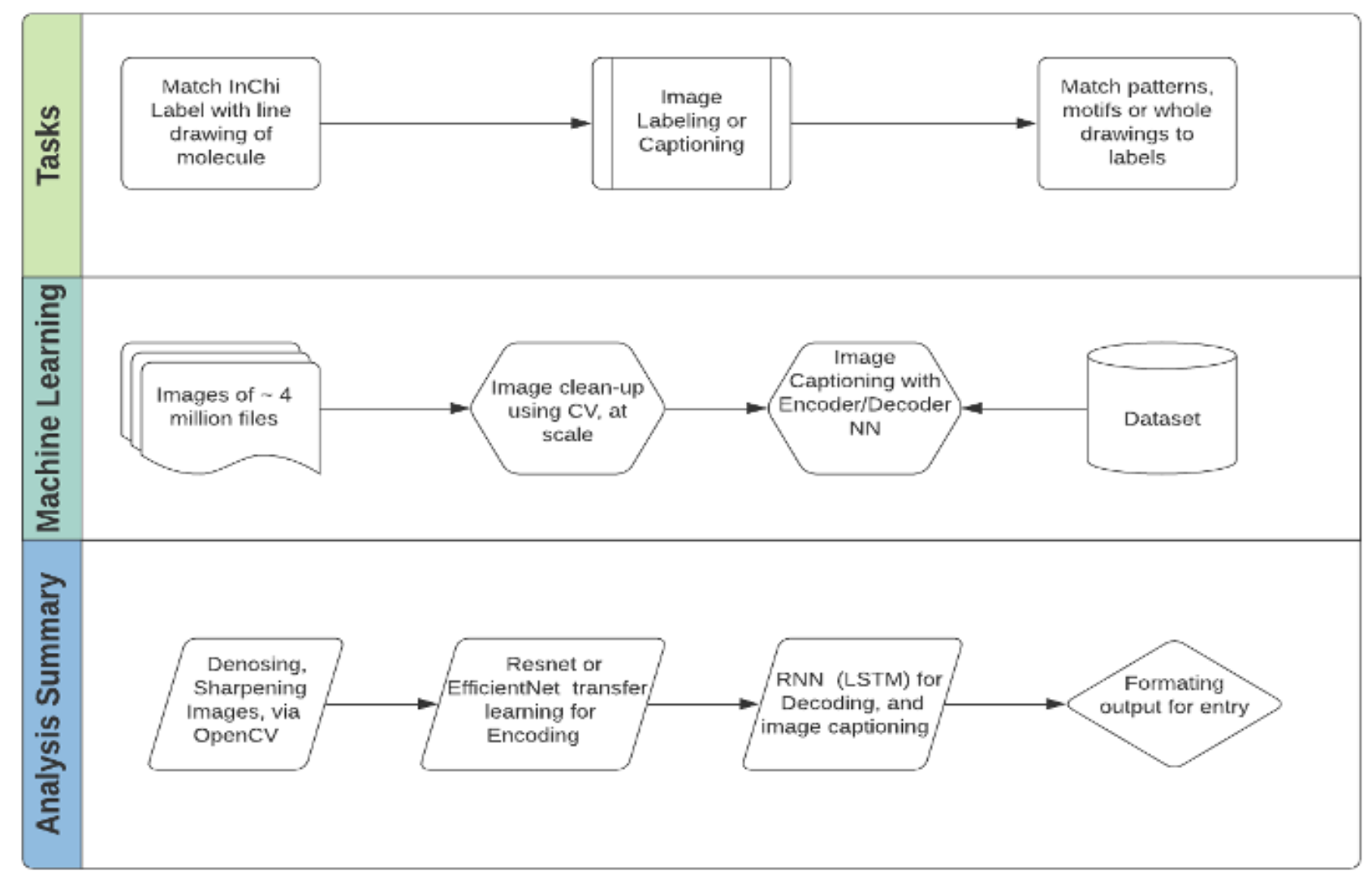
Figure 2: Process flow for creating image labeling system. Note: of the 2 million training samples, each image is a unique InChi and only represented once. However, images of the same molecule may be rotated, and are in fact, randomly rotated in the test dataset. For this reason, each image in the training set is represented only once. IC includes an encoder (transfer learning trained - basically done/coded up) and a decoder (RNN or LSTM) to create the 'caption' based on components of the image.
Our experimental plans changed early on in our process. Initially, we planned to leverage two advanced techniques for our training process. These included an attention mechanism and beam search. We found that it was not practical to optimize these two techniques while we optimized basic labeling experiments. Because our overall goal was to determine whether we could benchmark training time, we decided to leave out the activation function and beam search for our first experiment.
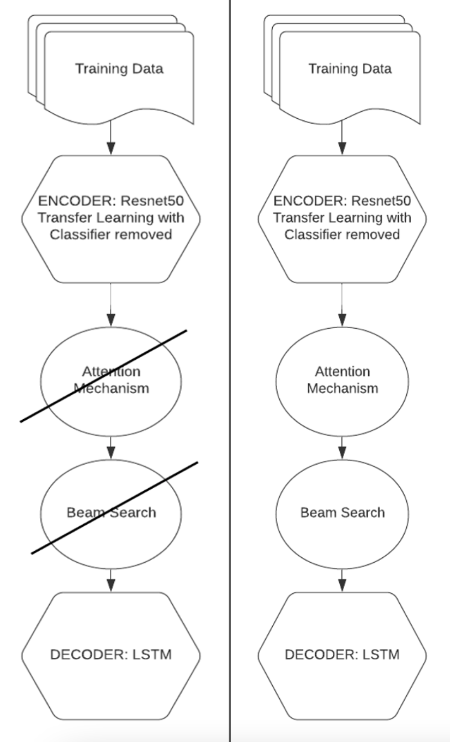
Figure 3: We originally intended to use an attention mechanism and beam search (advanced computer vision techniques). However, our first goal was to benchmark a canonical image labeling pipeline, so we decided to leave out the attention mechanism and beam search to focus solely on benchmarking with Ray. On the left is the algorithmic stack we decided to use and on the right is the original algorithmic stack.
Results
Our model was an elementary version of an image labeling pipeline, like that used in (Kishore, V, 2020). It was very close (missing only an attention mechanism) to the second-place winner of the Kaggle competition. This team's work took over seven days to train on a single GPU. We found that our training took about one and a half days, a significant decrease in time. While we did not use an attention mechanism, we did use the same data transfer learning mechanism with Resnet50, and an LSTM as our decoder.
In sum, our training pipeline included tokenization, an encoder using Resnet50, and a decoder leveraging an LSTM and significantly reduced training time. Running such experiments in the Domino Enterprise MLOps platform was very straightforward, as the system abstracted the infrastructure complexity, thus enabling us to utilize various CPU backend compute instances. Moreover, the self-service capabilities provided by Domino make it easy to install packages on the fly, and the out-of-the-box Ray supports makes it possible to spin up multi-node Ray clusters with a click of a button.
Future Experiments
In the future, we plan to replicate the process used by the second-place Kaggle winner by adding an attention mechanism to our pipeline. We will then test the use of Ray workers once again, this time using both CPUs and GPUs. We may also investigate the optimization of the techniques using beam search. For now, we focused on the advantages of speeding up training times.
References
- Second Place Winner’s Entry: https://www.kaggle.com/yasufuminakama/inchi-resnet-lstm-with-attention-starter
- 'Winning Solutions from Kaggle's Molecular Translation Hackathon,' June 17, 2021, URL: https://analyticsindiamag.com/winning-solutions-from-kaggles-molecular-translation-hackathon/
- Modern Computer Vision with Pytorch: Explore deep learning concepts and implement over 50 real-world image applications by V Kishore Ayyadevara and Yeshwanth Reddy, Packt Publishing, 2020.
- Deep Learning for Computer Vision: A Brief Review. Voulodimos A, Doulamis N, Doulamis A, Protopadakis, E. Computational Intelligence and Neuroscience, 2018.
RELATED TAGS
SHARE


Subscribe to the Domino Newsletter
Receive data science tips and tutorials from leading Data Science leaders, right to your inbox.
By submitting this form you agree to receive communications from Domino related to products and services in accordance with Domino's privacy policy and may opt-out at anytime.