Machine Learning Approach to Forecast Cars’ Demand
This article was published as a part of the Data Science Blogathon.
Introduction on Machine Learning
Last month, I participated in a Machine learning approach Hackathon hosted on Analytics Vidhya’s Datahack platform. Over a weekend, more than 600 participants competed to build and improve their solutions and climb the leaderboard. In this article, I will be sharing my hackathon experience – what worked, what didn’t work, and what I learned from it.
Objective of Machine Learning Approach
Forecasting the demand for car rentals on an hourly basis based on past data.
Loading and Exploring Data
Importing necessary libraries
%matplotlib inline
import numpy as np
import pandas as pd
import matplotlib.pyplot as plt
import seaborn as sns
import datetime as dt
from sklearn.metrics import mean_squared_error
Importing Train and Test Data
train_df = pd.read_csv('train_E1GspfA.csv')
test_df = pd.read_csv('test_6QvDdzb.csv')
Data Overview
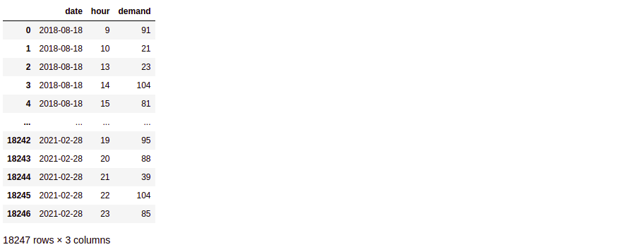
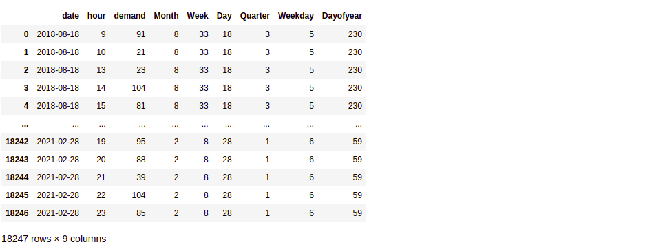
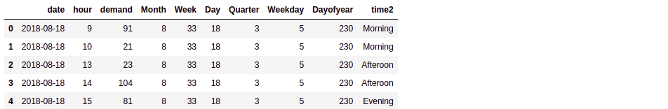
train_df.head()
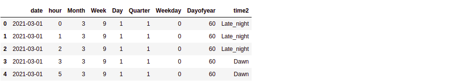
test_df.head()
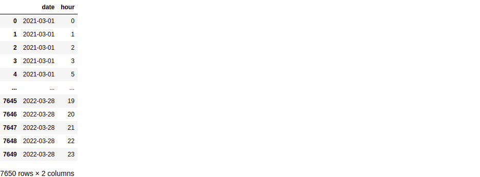
So basically, we are provided with the train data comprising of hourly rental car demand spanning from mid-Aug 2018 to Feb 2021 (approx 31 months). Our job is to make a prediction on the next 13 months of the test data (i.e. from Mar 2021 to Mar 2022).
Data Cleaning and Pre-processing
Check for the datatype of the data in the columns
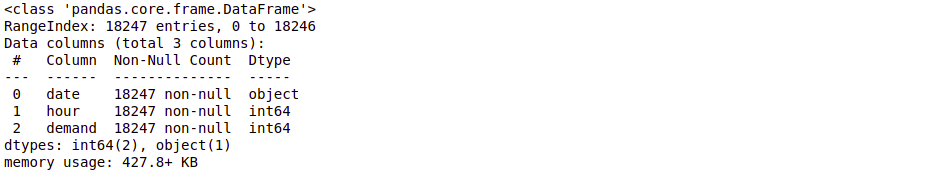
train_df.info()
test_df.info()
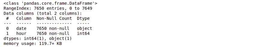
This also tells us that there are no null values in the data.
Check for duplicate entries
train_df.duplicated().sum()
As seen, no duplicate data is present.
From visual analysis, I believe that the train dataframe is already sorted, but let’s just do it.
Sorting dataframe by ‘date’ and ‘hour’ —
train_df = train_df.sort_values(by = ['date', 'hour'])
Now that we have organised the data, let’s proceed to the next stage.
Feature Engineering
As seen we don’t don’t really have many features. ‘hour’ data we already have, let’s see what information we can extract from the ‘date’ column
train_df['date'] = pd.to_datetime(train_df['date'])
train_df['Month'] = train_df.date.dt.month
train_df['Week'] = train_df.date.dt.week
train_df['Day'] = train_df.date.dt.day
train_df['Quarter'] = train_df.date.dt.quarter
train_df['Weekday'] = train_df.date.dt.dayofweek
train_df['Dayofyear'] = train_df.date.dt.dayofyear
This is how our dataframe looks after adding newly engineered features
train_df
Repeat same feature engineering steps on test data
test_df['date'] = pd.to_datetime(test_df['date'])
test_df['Month'] = test_df.date.dt.month
test_df['Week'] = test_df.date.dt.week
test_df['Day'] = test_df.date.dt.day
test_df['Quarter'] = test_df.date.dt.quarter
test_df['Weekday'] = test_df.date.dt.dayofweek
test_df['Dayofyear'] = test_df.date.dt.dayofyear
Note that here ‘Day’ means what day of the month it is, while ‘Dayofyear’, as the name suggests, represents what day of the year it is.
Now that we have extracted additional features from ‘date’, can we do something about the ‘hour’ feature? Can we somehow aggregate it to form a new feature?
Generating new feature ‘time2’ based on what part of the day the ‘hour’ falls in
def time_day(t):
    if t in [12, 13, 14]:
        return 'Afteroon'
    elif t in [15, 16, 17]:
        return 'Evening'
    elif t in [18, 19, 20]:
        return 'Late_evening'
    elif t in [21, 22, 23]:
        return 'Night'
    elif t in [0, 1, 2]:
        return 'Late_night'
    elif t in [3, 4, 5]:
        return 'Dawn'
    elif t in [6, 7, 8]:
        return 'Early_morning'
    elif t in [9, 10, 11]:
        return 'Morning'
train_df['time2'] = train_df['hour'].apply(lambda x:time_day(x))
test_df['time2'] = test_df['hour'].apply(lambda x:time_day(x))
So far we have extracted the following features from ‘date’ and ‘hour’ data – ‘Month’, ‘Week’, ‘Day’, ‘Quarter’, ‘Weekday’, ‘Dayofyear’, ‘time2’.
Since the beginning, we are assuming that it is possible to forecast the future demand based on the past data. But, can the past data really tell us about the future? Let’s test our hypothesis using Exploratory analysis.
Hypothesis testing – Exploratory Data Analysis
Let’s first divide our train data
1. From March’19 to February’20
2. From March’20 to February’21
# Mar-19 to Feb-20
train_df_19 = train_df[(train_df['date'] >= '01-03-2019') & (train_df['date'] <= '29-02-2020')]

# Mar-20 to Feb-21
train_df_20 = train_df[(train_df['date'] >= '01-03-2020') & (train_df['date'] <= '28-02-2021')]
Plotting demand by ‘Hour’, ‘Month’, ‘Week’, ‘Day’, ‘Quarter’, ‘Weekday’, ‘Dayofyear’, ‘time2’ —
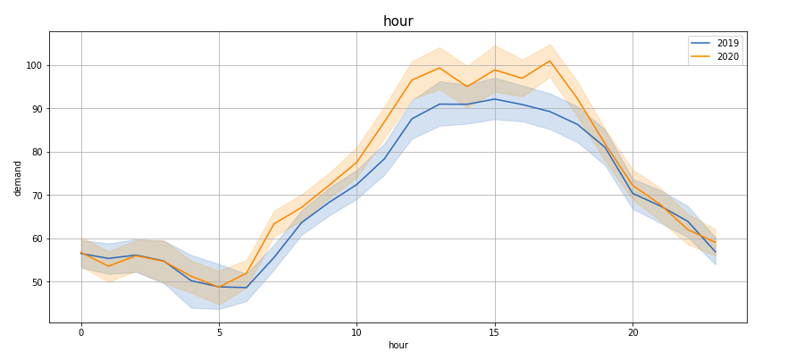
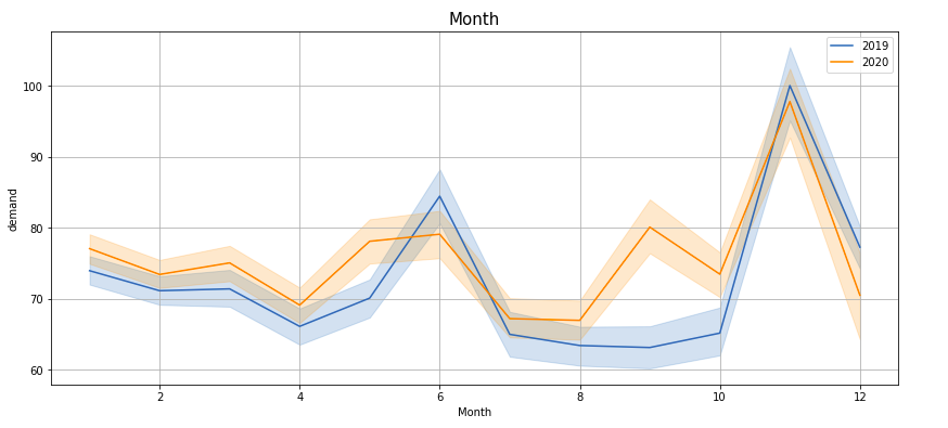
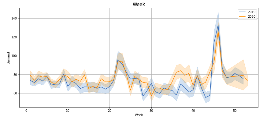
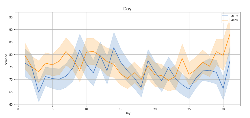
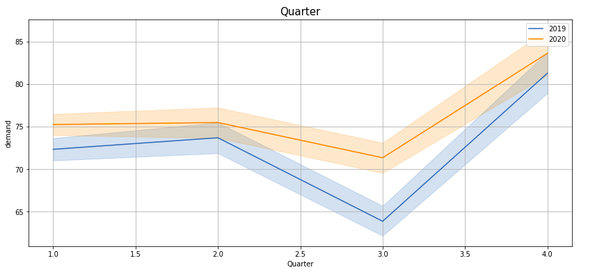
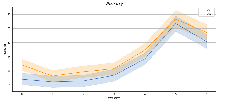
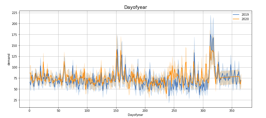
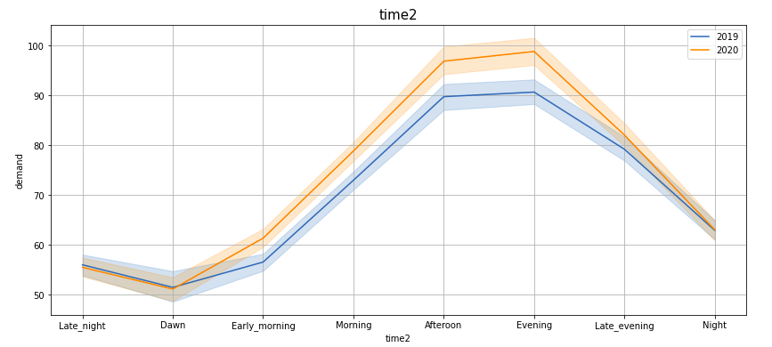
If you observe these lineplots, there is a lot of similarity in the demand trend in the years 2019 and 2020 (March to Feb). Especially if we see ‘Hour’, ‘Quarter’, ‘Weekday’, ‘Dayofyear’ and ‘time2’ plots, the peaks and troughs tend to concur.
Now that we are convinced that the newly engineered features along with the existing features can prove useful in predicting the demand for the subsequent year, let’s proceed to the modelling stage.
Hypothesis testing – Exploratory Data Analysis
Let’s observe our train and test data —
train_df.head()
test_df.head()
Drop redundant columns from train and test data —
X_train = train_df.drop(['date'], axis = 1)
X_test = test_df.drop(['date'], axis = 1)
y_train = train_df['demand']
Split training data further into training and validation data
from sklearn.model_selection import train_test_split
X_train, X_val, y_train, y_val = train_test_split(X_train, y_train, test_size = 0.30, shuffle = False)
print(X_train.shape, y_train.shape)
print(X_val.shape, y_val.shape)

Before we proceed, recall we had handcrafted a new variable ‘time2’? It is a categorical variable and machine learning models, in general, cannot consume categorical variables directly. So it needs to be encoded. We can do label encoding here, but usually, I do not prefer label encoding unless the variable has some inherent ordering. So what other option do we have? Let’s do response encoding!
Mean-encoding ‘time2’ variable
agg_df = pd.DataFrame(X_train.groupby(['time2']).agg({'demand':'mean'})).reset_index()
agg_df['demand'] = round(agg_df['demand'], 2)
agg_dict = dict(agg_df.values)
print(agg_dict)
X_train['time2'] = X_train['time2'].apply(lambda x:agg_dict[x])
X_val['time2'] = X_val['time2'].apply(lambda x:agg_dict[x])

The above dictionary represents the numerical values that these categorical variables take upon encoding.
Let’s train some tree-based ensembles and perform testing on the validation data in order to select the best model. The metric for scoring is Root mean-squared error (RMSE) —
from xgboost import XGBRegressor
from lightgbm import LGBMRegressor
from catboost import CatBoostRegressor
from sklearn.metrics import mean_squared_error
X_train = X_train.drop(['demand'], axis = 1)
X_val = X_val.drop(['demand'], axis = 1)
models = [XGBRegressor(), LGBMRegressor(), CatBoostRegressor()]
for model in models:
    model.fit(X_train, y_train)
    y_train_pred = model.predict(X_train)
    y_val_pred = model.predict(X_val)
    train_error = mean_squared_error(y_train, y_train_pred)
    validation_error = mean_squared_error(y_val, y_val_pred)
    print("Model: ", model)
    print("Train RMSE:", round(np.sqrt(train_error), 4))
    print("Validation RMSE:", round(np.sqrt(validation_error), 4))
| Train RMSE | Validation RMSE | ||
| XGBRegressor | 25.5833 | 37.9044 | |
| LGBMRegressor | 29.981 | 36.5979 | |
| CatBoostRegressor | 28.8737 | 36.6496 |
(Here I am displaying the result of the three models in the tabular format for the sake of brevity).
The comparative analysis of the performance of the models on the validation set reveals that the Light-GBM regressor model is the best among the three. So we select LGBMRegressor.
Now repeat all the above steps on the complete training dataset and make the prediction on the test dataset —
X_train = train_df.copy()
X_train = X_train.drop(['date'], axis = 1)
# encoding time2 variable
agg_df = pd.DataFrame(X_train.groupby(['time2']).agg({'demand':'mean'})).reset_index()
agg_df['demand'] = round(agg_df['demand'], 2)
agg_dict = dict(agg_df.values)
X_train['time2'] = X_train['time2'].apply(lambda x:agg_dict[x])
X_test['time2'] = X_test['time2'].apply(lambda x:agg_dict[x])
# lgbm regressor
y_train = X_train['demand']
X_train = X_train.drop(['demand'], axis = 1)
lgbm = LGBMRegressor()
lgbm.fit(X_train, y_train)
y_train_pred = lgbm.predict(X_train)
y_test_pred = lgbm.predict(X_test)
train_error = mean_squared_error(y_train, y_train_pred)
print("Train RMSE:", round(np.sqrt(train_error), 4))

Finally, make a submission with the predicted values —
submit_df = pd.read_csv('sample_4E0BhPN.csv')
submit_df['demand'] = y_test_pred
submit_df.to_csv('lgbm_baseline.csv', index = False)
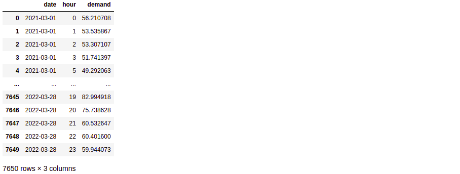
# display the submission file
submit_df
Post-Modelling Analysis
Let’s see what all features contributed towards predicting the rental cabs demand and their relative importance.
feat_df = pd.DataFrame({'Features': X_train.columns, 'Relative importance': lgbm.feature_importances_})
imp_feat_df = feat_df.sort_values('Relative importance', ascending = False)
plt.figure(figsize = (8, 6))
sns.barplot(x = 'Relative importance', y = 'Features', data = imp_feat_df)
plt.grid()
plt.show()
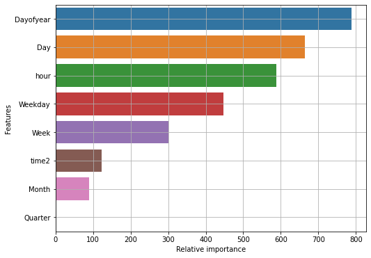
Turns out that ‘Dayofyear’ is the most important feature followed by ‘Day’ and ‘hour’. Also, the feature ‘Quarter’ is negligibly significant for our prediction task, so it can be discarded.
Conclusion on Machine learning
In the beginning, were provided with the hourly data of the Car rentals from mid-Aug 2018 to Feb 2021. We did some high-level analysis, followed by feature engineering. Using newly extracted features we tested our hypothesis by performing exploratory analysis. Then finally we trained a regression model to predict the hourly demand of the rental Cars from Mar 2021 to Mar 2022.
Key Takeaways on machine learning
- Feature engineering is good and can drastically improve the model performance, but overdoing it can lead to overfitting resulting in bad performance on the test data.
- Make sure you keep train and test (or validation) data separate while encoding categorical variables to avoid data leakage issues.
- The rank on the public leaderboard is often deceptive. Here your prediction is evaluated partially so you may end up with a sub-optimal model. Always make sure you test your models on validation data first before deciding which model to finalize.
- Here we used all baseline models. So once the best model is selected, we can try hyperparameter tuning to see if the model performance improves further.
The media shown in this article is not owned by Analytics Vidhya and is used at the Author’s discretion.


