Pokemon Prediction using Random Forest
This article was published as a part of the Data Science Blogathon
Overview
This Pokemon will analyze the pokemon dataset and predict whether the Pokemon is legendary based on the features provided. We will discuss everything from scratch; we will go from CSV to model building with line by line explanation of code. Let’s get started.

Image source: Pokejungle
Takeaways
- Understand how to analyze the dataset before carrying forward to the model building phase.
- Getting the insights from the data.
- Visualization of the dataset.
- Model building
- Saving model.
About the dataset
This dataset has 721 unique values i.e. it has features of 721 unique pokemon; for further details, visit this link.
.png)
Importing necessary libraries
import pandas as pd
import numpy as np
import seaborn as sns
import matplotlib.pyplot as plt
%matplotlib inline

from sklearn.model_selection import train_test_split
from sklearn.metrics import accuracy_score, classification_report
from sklearn.ensemble import RandomForestClassifier
Reading the dataset
pokemon_data = pd.read_csv('Pokemon Data.csv')
Now, let’s see what our dataset has in it!
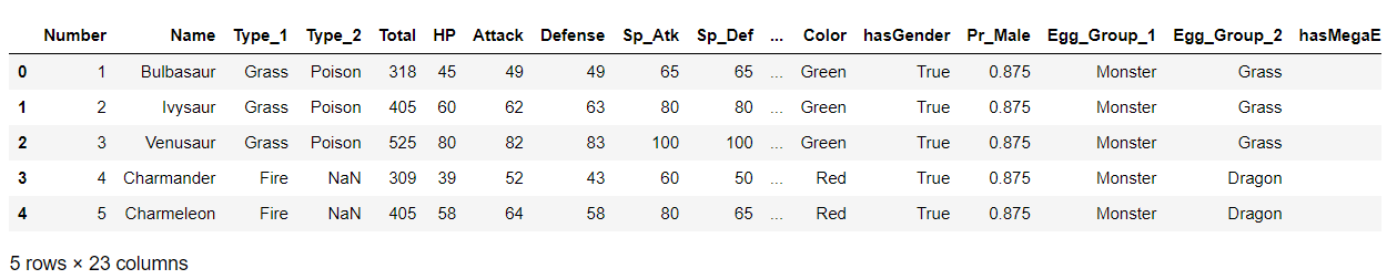
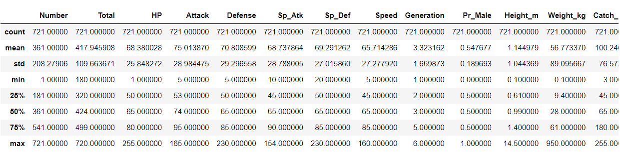
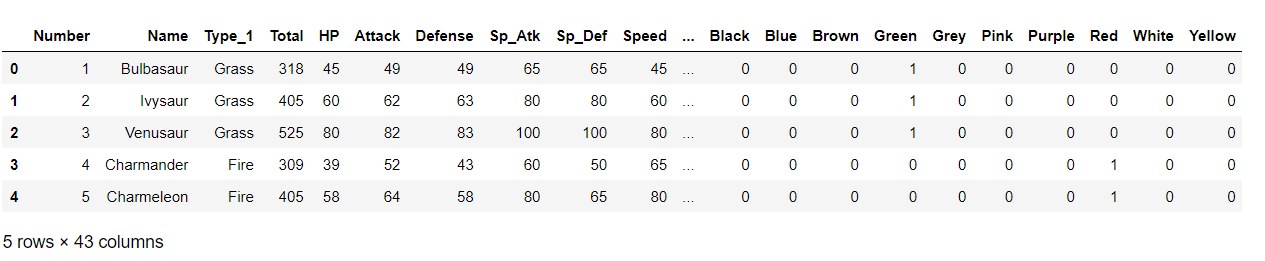
poke = pd.DataFrame(pokemon_data)
poke.head()
Output:
Checking out folet’sl values
poke.isnull().sum()
Output:
Number                0
Name                  0
Type_1                0
Type_2              371
Total                 0
HP                    0
Attack                0
Defense               0
Sp_Atk                0
Sp_Def                0
Speed                 0
Generation            0
isLegendary           0
Color                 0
hasGender             0
Pr_Male              77
Egg_Group_1           0
Egg_Group_2         530
hasMegaEvolution      0
Height_m              0
Weight_kg             0
Catch_Rate            0
Body_Style            0
dtype: int64
We have seen the null values in its users n; let’s visualize them using the heatmap.
plt.figure(figsize=(10,7))
sns.heatmap(poke.isnull(), cbar=False)
Output:
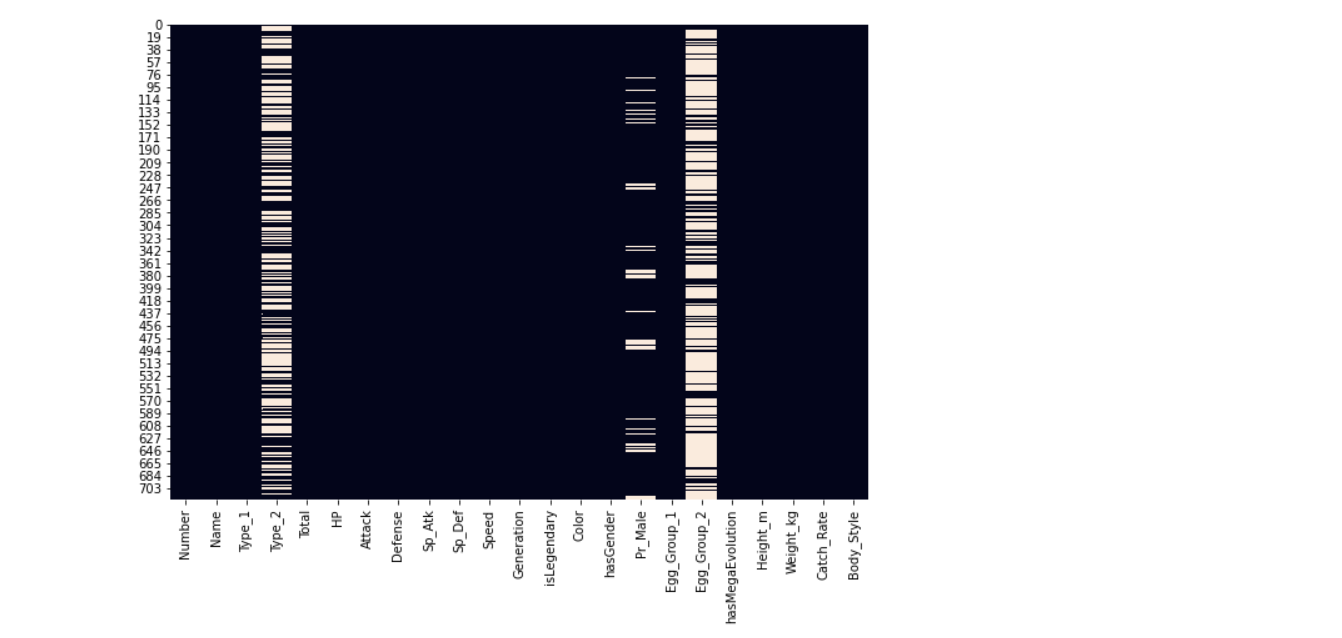
Here it’s visible that Type_2, Pr_Male, and Egg_Group_2 have relatively null values.
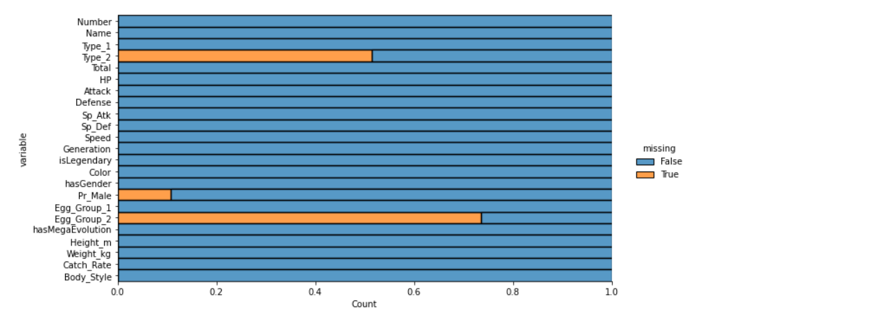
We have visualized the nucan’tlues using the heatmap but in that kind of visualization, we can’t get the count of Let’s null values, so we are using the dist-plot.
plt.figure(figsize=(20,20))
sns.displot(
    data=poke.isna().melt(value_name="missing"),
    y="variable",
    hue="missing",
    multiple="fill",
    aspect=2
)
Output:
Let’s know the dimensions of our dataset.
poke.shape
Output:
(721, 23)
From the shape, it is clear the dataset is small, meaning we can remove the null values columns as filling them can make the dataset a little biased.
We have seen that type_2, egg_group_2, and Pr_male have null values.
poke['Pr_Male'].value_counts()
Output:
0.500    458
0.875    101
0.000     23
0.250     22
0.750     19
1.000     19
0.125      2
Name: Pr_Male, dtype: int64
Since Type_2 and Egg_group_2 columns have so many NULL values we will be removing those columns, you won’t impute them with other methods, but for simplicity, we won’t do that here. We only set the Pr_Male column since it had only 77 missing values.
poke['Pr_Male'].fillna(0.500, inplace=True)
poke['Pr_Male'].isnull().sum()
Output:
0 # as we can see that there are no null values now.
Dropping unnecessary columns
new_poke = poke.drop(['Type_2', 'Egg_Group_2'], axis=1)
Now let’s understand the type of each column and its values.
new_poke.describe()
Note : (20, 20000) -> x -min/ max-min -> x = 300 -> 300-20/19980 -> a very small value
Output:
plt.figure(figsize=(10,10))
sns.heatmap(new_poke.corr(),annot=True,cmap='viridis',linewidths=.5)
Output:
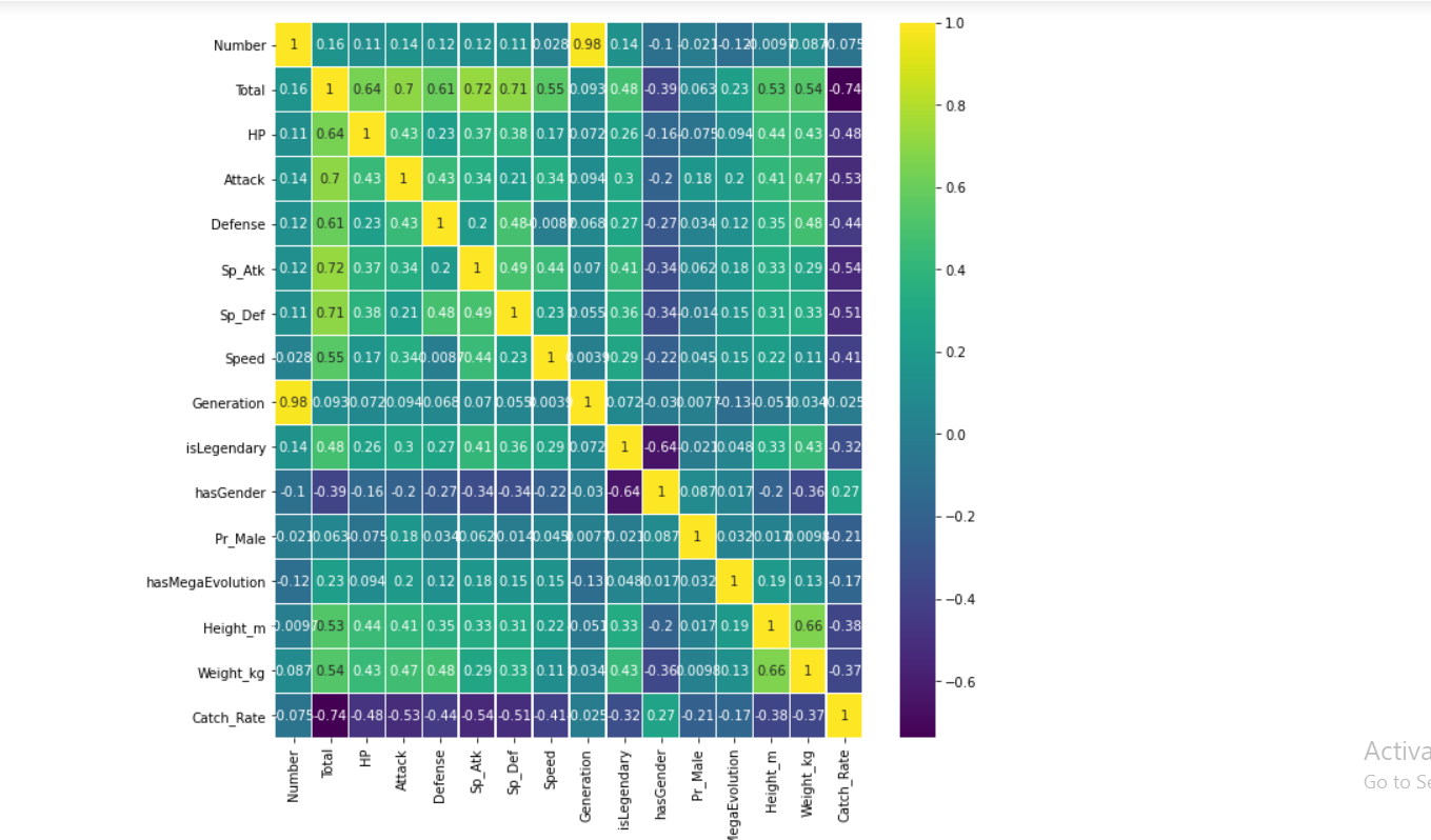
- The above is a correlation graph that tells you how much a feature is correlated to another since a high correlation means one of the two features does not speak much to the model when predicting.
- Usually, it is to be determined by you itself for the high value of correlation and removed.
- From the above table, it is clear that different features have different ranges of value, which creates complexity for the model, so we tone them down usually using StandardScalar() class which we will do later on.
new_poke['Type_1'].value_counts()
Output:
Water       105
Normal       93
Grass        66
Bug          63
Psychic      47
Fire         47
Rock         41
Electric     36
Ground       30
Poison       28
Dark         28
Fighting     25
Dragon       24
Ice          23
Ghost        23
Steel        22
Fairy        17
Flying        3
Name: Type_1, dtype: int64
Value counts of all the generations
new_poke['Generation'].value_counts()
Output:
5    156
1    151
3    135
4    107
2    100
6     72
Name: Generation, dtype: int64
Visualizing I’me categorical values
Here for visualizing the categorical data, I’m using seaborn’s cat plot() function. Well, one can use the line plot scatter plot or box plot separately, but here, the cat plot brings up the unified version of using all the plots hence I preferred the cat plot rather than the separate version of eI’m plot.
Here for counting each type (6) category of generations, I’m using the cougeneration’snd in the cat plot to get the number of count of each generation’s column.
sns.catplot(x="Generation",kind="count",palette="ch:.25", data=poke)
Output:
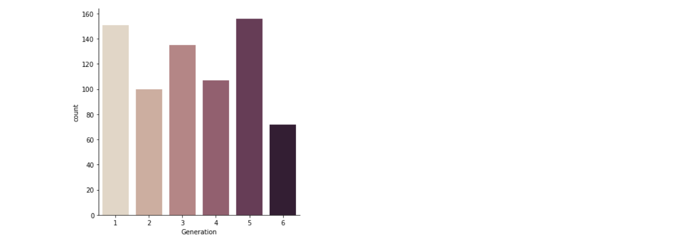
Inference: In the above graph, the 5th generation is the most in numbers.
Here we are using the default kind of cat plot, i.e. scatter plot to plot the Generation vs Defense graph where we will be able to figure outPokemonlationship between the defence power of each general Pokemon.
sns.catplot(x="Generation", y="Defense", data=poke)
Output:
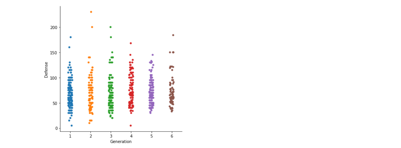
Inference: Here, we can see that only two pcan’tn in generation 2 have the highest defence capability. Still, we can’t conclude that generation 2 has the most increased defence capabilities as the outliers. Still, in the graph, it is evident that generation 6 and 4 has the highest defence capabilities.
Here we are using the Box plot because boxplot will help us understand the variations in the large dataset better; it will also let us know about the outliers more clearly.
sns.catplot(x="Generation", y="Attack",kind="boxen", data=poke)
Output:
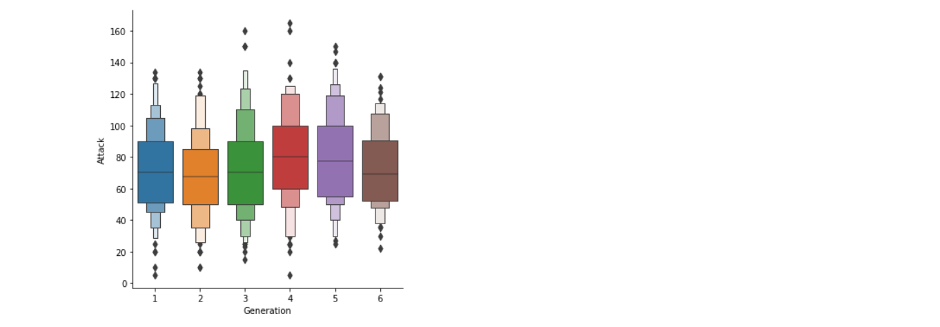
- Here in the above boxplot, we can see that there are a lot of outliers in generation 4 and generation 1 when it comes to attacking capabilities.
- Also, generation 4 has the highest median values of their attacking capabilities than all the other generations.
Now we are using bar kind via cat plot, which will let us know about the Attacking capabilities of different generations based on their Pokemon. For example, in generation 1, the pokemon power of male Pokemon are higher than those of the female Pokemon of the same generation. Still, that generation also has the least attacking power than other generations.
sns.catplot(x="Generation", y="Attack",kind='bar',hue='hasGender', data=poke)
Output:
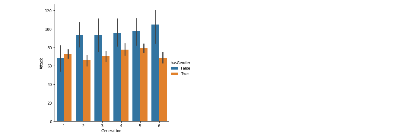
FromPokemonove graph, we can conclude that,
- In generaPokemononly the male Pokemon has more attacking power than the female Pokemon, which contradicts other generations.
- Generation 6 has the highest attacking power wLet’sgeneration 1 has the lowest attacking power.
new_poke['Color'].value_counts()
Output:
Blue      134
Brown     110
Green      79
Red        75
Grey       69
Purple     65
Yellow     64
White      52
Pink       41
Black      32
Name: Color, dtype: int64

new_poke['Egg_Group_1'].value_counts()
Output:
Field           169
Monster          74
Water_1          74
Undiscovered     73
Bug              66
Mineral          46
Flying           44
Amorphous        41
Human-Like       37
Fairy            30
Grass            27
Water_2          15
Water_3          14
Dragon           10
Ditto             1
Name: Egg_Group_1, dtype: int64
Let’s also consider the number of values in our target column
new_poke['isLegendary'].value_counts()
Output:
False    675
True      46
Name: isLegendary, dtype: int64
Feature Engineering
Creating new categories or merging categories, so it is easy to work with afterwards.
This may seem uncomfortable to some, but you will get why I did it like that.
poke_type1 = new_poke.replace(['Water', 'Ice'], 'Water')
poke_type1 = poke_type1.replace(['Grass', 'Bug'], 'Grass')
poke_type1 = poke_type1.replace(['Ground', 'Rock'], 'Rock')
poke_type1 = poke_type1.replace(['Psychic', 'Dark', 'Ghost', 'Fairy'], 'Dark')
poke_type1 = poke_type1.replace(['Electric', 'Steel'], 'Electric')
poke_type1['Type_1'].value_counts()
Output:
Grass       129
Water       128
Dark        115
Normal       93
Rock         71
Electric     58
Fire         47
Poison       28
Fighting     25
Dragon       24
Flying        3
Name: Type_1, dtype: int64
ref1 = dict(poke_type1['Body_Style'].value_counts())

poke_type1['Body_Style_new'] = poke_type1['Body_Style'].map(ref1)
You may be wondering what I did; I took the value counts of each body tyLet’sd replace the body type with the numbers; see below
poke_type1['Body_Style_new'].head()
Output:
0    135
1    135
2    135
3    158
4    158
Name: Body_Style_new, dtype: int64
Let’s look towards the Body_style
poke_type1['Body_Style'].head()
Output:
0         quadruped
1         quadruped
2         quadruped
3    bipedal_tailed
4    bipedal_tailed
Name: Body_Style, dtype: object
Encoding data – features like Type_1 and Color
types_poke = pd.get_dummies(poke_type1['Type_1'])
color_poke = pd.get_dummies(poke_type1['Color'])

X = pd.concat([poke_type1, types_poke], axis=1)
X = pd.concat([X, color_poke], axis=1)

X.head()
Output:
Now we have built some features and extracted some feature data, what’s left is to remove redundant features
X.columns
Output:
Index(['Number', 'Name', 'Type_1', 'Total', 'HP', 'Attack', 'Defense',
       'Sp_Atk', 'Sp_Def', 'Speed', 'Generation', 'isLegendary', 'Color',
       'hasGender', 'Pr_Male', 'Egg_Group_1', 'hasMegaEvolution', 'Height_m',
       'Weight_kg', 'Catch_Rate', 'Body_Style', 'Body_Style_new', 'Dark',
       'Dragon', 'Electric', 'Fighting', 'Fire', 'Flying', 'Grass', 'Normal',
       'Poison', 'Rock', 'Water', 'Black', 'Blue', 'Brown', 'Green', 'Grey',
       'Pink', 'Purple', 'Red', 'White', 'Yellow'],
      dtype='object')
X_ = X.drop([‘Number’, ‘Name’, ‘let’s1’, ‘Color’, ‘Egg_Group_1’], axis = 1)
X_.shape
Output:
(721, 38)
Now, let’s see the shape of our updated feature columns
X.shape
Lastly, we define our target variable and set it into a variable called y
y = X_['isLegendary']
X_final = X_.drop(['isLegendary', 'Body_Style'], axis = 1)
X_final.columns
Output:
Index(['Total', 'HP', 'Attack', 'Defense', 'Sp_Atk', 'Sp_Def', 'Speed',
       'Generation', 'hasGender', 'Pr_Male', 'hasMegaEvolution', 'Height_m',
       'Weight_kg', 'Catch_Rate', 'Body_Style_new', 'Dark', 'Dragon',
       'Electric', 'Fighting', 'Fire', 'Flying', 'Grass', 'Normal', 'Poison',
       'Rock', 'Water', 'Black', 'Blue', 'Brown', 'Green', 'Grey', 'Pink',
       'Purple', 'Red', 'White', 'Yellow'],
      dtype='object')
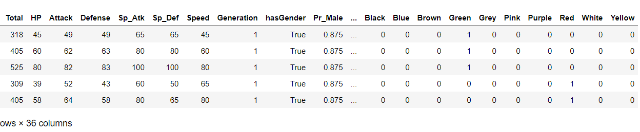
X_final.head()
Output:
Creating and training our model
Splitting the dataset into training and testing dataset
Xtrain, Xtest, ytrain, ytest = train_test_split(X_final, y, test_size=0.2)
Using random forest classifier for training our model
random_model = RandomForestClassifier(n_estimators=500, random_state = 42)
Fitting the model
model_final = random_model.fit(Xtrain, ytrain)
y_pred = model_final.predict(Xtest)
Checking the accuracy
random_model_accuracy = round(model_final.score(Xtrain, ytrain)*100,2)
print(round(random_model_accuracy, 2), '%')
Output:
100.0 %
Getting the accuracy of the model
random_model_accuracy1 = round(random_model.score(Xtest, ytest)*100,2)
print(round(random_model_accuracy1, 2), '%')
Output:
99.31 %
Saving the model to disk
import pickle
filename = 'pokemon_model.pickle'
pickle.dump(model_final, open(filename, 'wb'))
Load the model from the disk
filename = 'pokemon_model.pickle'
loaded_model = pickle.load(open(filename, 'rb'))
result = loaded_model.score(Xtest, ytest)

result*100
Output:
99.3103448275862
Conclusion
Here I conclude the legendary pokemon prediction with 99% accuracy; this might be a overfit model; having said that, the dataset was not so complex that it will lead to such a situaHere’set all the suggestions and improvements are always welcome.
Here’s the repo link to this article.
Here you can access my other articles, which are published on Analytics Vidhya as a part of the Blogathon (link)
If got any queries you can connect with I’m on LinkedIn, refer to this link
About me
Greeting to everyone, I’m currently working in TCS and previously, I worked as a Data Science AssociI’veAnalyst in Zorba Consulting India. Along with full-time work, I’ve got an immense interest in the same field, i.e. Data Science, along with its other subsets of Artificial Intelligence such as Computer Vision, Machine learning, and Deep learning; feel free to collaborate with me on any project on the domains mentioned above (LinkedIn).
The media shown in this article is not owned by Analytics Vidhya and are used at the Author’s discretion.


