Speed up queries with the cost-based optimizer in Amazon Athena

Amazon Athena is a serverless, interactive analytics service built on open source frameworks, supporting open table file formats. Athena provides a simplified, flexible way to analyze petabytes of data where it lives. You can analyze data or build applications from an Amazon Simple Storage Service (Amazon S3) data lake and 30 data sources, including on-premises data sources or other cloud systems using SQL or Python. Athena is built on open source Trino and Presto engines and Apache Spark frameworks, with no provisioning or configuration effort required.

Starting today, the Athena SQL engine uses a cost-based optimizer (CBO), a new feature that uses table and column statistics stored in the AWS Glue Data Catalog as part of the table’s metadata. By using these statistics, CBO improves query run plans and boosts the performance of queries run in Athena. Some of the specific optimizations CBO can employ include join reordering and pushing aggregations down based on the statistics available for each table and column.

TPC-DS benchmarks These benchmarks demonstrate the power of the cost-based optimizer—queries run up to 2x times faster with CBO enabled compared to running the same TPC-DS queries without CBO.

Performance and cost comparison on TPC-DS benchmarks

We used the industry-standard TPC-DS 3 TB to represent different customer use cases. These are representative of workloads with 10 times the stated benchmark size. This means a 3 TB benchmark dataset accurately represents customer workloads on 30–50 TB datasets.

In our testing, the dataset was stored in Amazon S3 in non-compressed Parquet format and the AWS Glue Data Catalog was used to store metadata for databases and tables. Fact tables were partitioned on the date column used for join operations, and each fact table consisted of 2,000 partitions. To help illustrate the performance of CBO, we compare the behavior of various queries and highlight the performance differences between running with CBO enabled vs. disabled.

The following graph illustrates the runtime of queries on the engine with and without CBO.

The following graph presents the top 10 queries from the TPC-DS benchmark with the greatest performance improvement.

Let’s discuss some of the cost-based optimization techniques that contributed to improved query performance.

Cost-based join reordering

Join reordering, an optimization technique used by cost-based SQL optimizers, analyzes different join sequences to select the order that minimizes query runtime by reducing intermediate data processed at each step, lowering memory and CPU requirements.

Let’s talk about query 82 of the TPC-DS 3TB dataset. The query performs inner joins on four tables: item, inventory, date_dim, and store_sales. The store_sales table has 8.6 billion rows and is partitioned by date. The inventory table has 1 billion rows and is also partitioned by date. The item table contains 360,000 rows, and the date_dim table holds 73,000 rows.

Query 82

select  i_item_id ,i_item_desc ,i_current_price
from item, inventory, date_dim, store_sales
where i_current_price between 30 and 30+30
and inv_item_sk = i_item_sk
and d_date_sk=inv_date_sk
and cast(d_date as date) between cast('2002-05-30' as date) and (cast('2002-05-30' as date) +  interval '60' day)
and i_manufact_id in (437,129,727,663)
and inv_quantity_on_hand between 100 and 500
and ss_item_sk = i_item_sk
group by i_item_id,i_item_desc,i_current_price
order by i_item_id
limit 100

Without CBO

Without using CBO, the engine will determine the join order based on the sequence of tables defined in the input query with internal heuristics. The FROM clause of the input query is "from item, inventory, date_dim, store_sales" (all inner joins). After passing through internal heuristics, Athena chose the join order as ((item ⋈ (inventory ⋈ date_dim)) ⋈ store_sales). Despite store_sales being the largest fact table, it’s defined last in the FROM clause and therefore gets joined last. This plan fails to reduce the intermediate join sizes as early as possible, resulting in an increased query runtime. The following diagram shows the join order without CBO and the number of rows flowing through different stages.

With CBO

When using CBO, the optimizer determines the best join order using a variety of data, including statistics as well as join size estimation, join build side, and join type. In this instance, Athena’s selected join order is ((store_sales ⋈ item) ⋈ (inventory ⋈ date_dim)). The largest fact table, store_sales, without being shuffled, is first joined with the item dimension table. The other partitioned table, inventory, is also first joined in-place with the date_dim dimension table. The join with the dimension table acts as a filter on the fact table, which dramatically reduces the input data size of the join that follows. Note that which side a table resides for a join is significant in Athena, because it’s the table on the right that will be built into memory for the join operation. Therefore, we always want to keep the larger table on the left and the smaller table on the right. CBO chose a plan that the left side was 8.6 billion before, and now it’s 13.6 million.

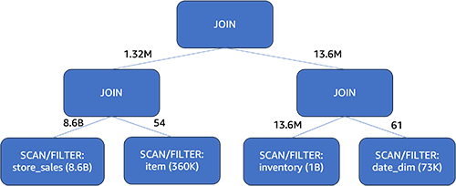
With CBO, the query runtime improved by 25% (from 15 seconds down to 11 seconds) by choosing the optimal join order.

Next, let’s discuss another CBO technique.

Cost-based aggregation pushdown

Aggregation pushdown is an optimization technique used by query optimizers to improve performance. It involves pushing aggregation operations like SUM, COUNT, and AVG into an earlier stage in the query plan, while maintaining the same query semantics. This reduces the amount of data transferred between the stages. By minimizing data processing, aggregation pushdown decreases memory usage, I/O costs, and network traffic.

However, pushing down aggregation is not always beneficial. It depends on the data distribution. For example, grouping on a column with many rows but few distinct values (like gender) before joins works better. Grouping first means aggregating a large number of records into fewer records (just male, female, for example). Grouping after joining means a large number of records have to participate the join before being aggregated. On the other hand, grouping on a high cardinality column is better done after joins. Doing it before risks unnecessary aggregation overhead because each value is likely unique anyway and that step will not result in an earlier reduction in the amount of data transferred between intermediate stages.

Therefore, whether to push down aggregation should be a cost-based decision. Let’s take example of the query 2 run on a 3TB TPC-DS dataset, showing how the aggregation pushdown’s value depends on data distribution. The web_sales table has 2.1 billion rows and the catalog_sales table has 4.23 billion rows. Both tables are partitioned on the date column.

Query 2

with wscs as
 (select sold_date_sk
        ,sales_price
  from (select ws_sold_date_sk sold_date_sk
              ,ws_ext_sales_price sales_price
        from web_sales 
        union all
        select cs_sold_date_sk sold_date_sk
              ,cs_ext_sales_price sales_price
        from catalog_sales)),
 wswscs as 
 (select d_week_seq,
        sum(case when (d_day_name='Sunday') then sales_price else null end) sun_sales,
        sum(case when (d_day_name='Monday') then sales_price else null end) mon_sales,
        sum(case when (d_day_name='Tuesday') then sales_price else  null end) tue_sales,
        sum(case when (d_day_name='Wednesday') then sales_price else null end) wed_sales,
        sum(case when (d_day_name='Thursday') then sales_price else null end) thu_sales,
        sum(case when (d_day_name='Friday') then sales_price else null end) fri_sales,
        sum(case when (d_day_name='Saturday') then sales_price else null end) sat_sales
 from wscs
     ,date_dim
 where d_date_sk = sold_date_sk
 group by d_week_seq)
 select d_week_seq1
       ,round(sun_sales1/sun_sales2,2)
       ,round(mon_sales1/mon_sales2,2)
       ,round(tue_sales1/tue_sales2,2)
       ,round(wed_sales1/wed_sales2,2)
       ,round(thu_sales1/thu_sales2,2)
       ,round(fri_sales1/fri_sales2,2)
       ,round(sat_sales1/sat_sales2,2)
 from
 (select wswscs.d_week_seq d_week_seq1
        ,sun_sales sun_sales1
        ,mon_sales mon_sales1
        ,tue_sales tue_sales1
        ,wed_sales wed_sales1
        ,thu_sales thu_sales1
        ,fri_sales fri_sales1
        ,sat_sales sat_sales1
  from wswscs,date_dim 
  where date_dim.d_week_seq = wswscs.d_week_seq and
        d_year = 2001) y,
 (select wswscs.d_week_seq d_week_seq2
        ,sun_sales sun_sales2
        ,mon_sales mon_sales2
        ,tue_sales tue_sales2
        ,wed_sales wed_sales2
        ,thu_sales thu_sales2
        ,fri_sales fri_sales2
        ,sat_sales sat_sales2
  from wswscs
      ,date_dim 
  where date_dim.d_week_seq = wswscs.d_week_seq and
        d_year = 2001+1) z
 where d_week_seq1=d_week_seq2-53
 order by d_week_seq1

Without CBO

Athena first joins the result of the union all operation on the web_sales table and the catalog_sales table with another table. Only then does it perform aggregation on the joined results. In this example, the amount of data that needed to be joined was huge, resulting in a longer query runtime.

With CBO

Athena utilizes one of the statistics values, the distinct value count, to evaluate the cost implications of pushing down the aggregation vs. not doing so. When a column has many rows but few distinct values, CBO is more likely to push aggregation down. This shrank the qualified rows from web_sales and catalog_sales tables to 2,590 and 3,590 rows, respectively. These aggregated records were then unioned and used to join with the tables. Comparing to the plan without CBO, the records participating in the join from the two large tables dropped from 6.33 billion rows (2.1 billion + 4.23 billion) to just 6,180 rows (2,590 + 3,590). This significantly decreased query runtime.

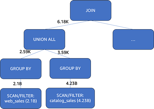
With CBO, the query runtime improved by 50% (from 37 seconds down to 18 seconds). In summary, CBO helped Athena choose an optimal aggregation pushdown plan, cutting the query time in half compared to not using cost-based optimization.

Conclusion

In this post, we discussed how Athena uses a cost-based optimizer (CBO) in its engine v3 to use table statistics for generating more efficient query run plans. Testing on the TPC-DS benchmark showed an 11% improvement in overall query performance when using CBO compared to without it.

Two key optimization employed by CBO are join reordering and aggregate pushdown. Join reordering reduces intermediate data by intelligently picking the order to join tables based on statistics. Aggregate pushdown decreases intermediate data by pushing aggregations earlier in the plan when beneficial.

In summary, Athena’s new cost-based optimizer significantly speeds up queries by choosing superior run plans. CBO optimizes based on table statistics stored in the AWS Glue Data Catalog. This automatic optimization improves productivity for Athena users through more responsive query performance. To take advantage of optimization techniques of CBO, refer to working with column statistics to generate statistics on the tables and columns in the AWS Glue Data Catalog.

About the Authors

Darshit Thakkar is a Technical Product Manager with AWS and works with the Amazon Athena team based out of Boston, Massachusetts.

Wei Zheng is a Sr. Software Development Engineer with Amazon Athena. He joined AWS in 2021 and has been working on multiple performance improvements on Athena.

Chuho Chang is a Software Development Engineer with Amazon Athena. He has been working on query optimizers for over a decade.

Pathik Shah is a Sr. Analytics Architect on Amazon Athena. He joined AWS in 2015 and has been focusing in the big data analytics space since then, helping customers build scalable and robust solutions using AWS analytics services.