Image Classification using Machine Learning

This article was published as a part of the Data Science Blogathon.

Dear readers,

In this blog, we will be discussing how to perform image classification using four popular machine learning algorithms namely, Random Forest Classifier, KNN, Decision Tree Classifier, and Naive Bayes classifier. We will directly jump into implementation step-by-step.

At the end of the article, you will understand why Deep Learning is preferred for image classification. However, the work demonstrated here will help serve research purposes if one desires to compare their CNN image classifier model with some machine learning algorithms.

So, let’s begin…

Agenda

• Dataset Acquisition
• Dataset Pre-processing
• Implementing a Random Forest Classifier
• Implementing a KNN
• Implementing a Decision Tree classifier
• Implementing a Naive Bayes classifier
• Results
• Testing for Custom input
• Conclusion

Dataset Acquisition

Source

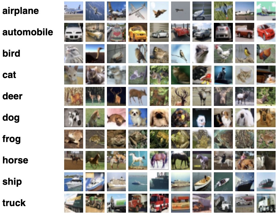
The dataset used in this blog is the CIFAR-10 dataset. It is a Keras dataset and thus can be directly downloaded from here with a simple code!It consists of ten classes, namely,airplane, automobile,bird,cat,deer,dog,frog,horse,ship and truck.Clearly, we will be working on a multi-class classification problem.

First, let’s import the required packages as follows:

from tensorflow import keras
import matplotlib.pyplot as plt

from sklearn.metrics import accuracy_score,confusion_matrix,classification_report
import numpy as np

import cv2

The dataset can be loaded using the code below:

(x_train, y_train), (x_test, y_test) = keras.datasets.cifar10.load_data()

Further, we can obtain the size of the train and test datasets as shown below:

x_train.shape,x_test.shape

Thus, there is a total of 50,000 images for training and 10,000 images for testing. Besides, each of these images is of dimensions 32×32 and colour. The above details can be easily inferred from the shape returned.

NOTE: Observe that there is no need for a train-test-split in this case as train and test sets can be directly obtained from Keras!

Dataset Pre-Processing

This step includes the normalization of images followed by their reshaping.

Normalization is a common step of image pre-processing and is achieved by simply dividing x_train by 255.0 for the train dataset and x_test by 255.0 for the test dataset. This is essential to maintain the pixels of all the images within a uniform range.

# Normalization
x_train = x_train/255.0
x_test = x_test/255.0

Now comes the most essential step of pre-processing, which is applicable only in this case as we aim to use machine learning for image classification. As we will be using the ML algorithms from sklearn, there is a need to reshape the images of the dataset to a two-dimensional array. This is because sklearn expects a 2D array as input to the fit() function which will be called on the model during training.

Thus, the images of the test dataset should also be resized to 2D arrays as the model was trained with this input shape.

NOTE: In the case of neural networks, we get to specify the input shape to the model and thus it is more flexible. But, in the case of sklearn, there are some restrictions.

The required code for the train set is as follows:

#sklearn expects i/p to be 2d array-model.fit(x_train,y_train)=>reshape to 2d array
nsamples, nx, ny, nrgb = x_train.shape
x_train2 = x_train.reshape((nsamples,nx*ny*nrgb))

The above code reshapes train set images from (50000,32,32,3) which is a 4D array to (50000,3072), a 2D array.3072 is obtained by multiplying the dimensions of the image(32x32x3=3072).

The required code for the test set is given below:

#so,eventually,model.predict() should also be a 2d input
nsamples, nx, ny, nrgb = x_test.shape
x_test2 = x_test.reshape((nsamples,nx*ny*nrgb))

from sklearn.ensemble import RandomForestClassifier

Create an instance of the RandomForestClassifier class:

model=RandomForestClassifier()

Finally, let us proceed to train the model:

model.fit(x_train2,y_train)

NOTE: Pass x_train2 to fit() function as it is the reshaped 2D array of the images and sklearn needs a 2D array as input here. Do this while fitting for all the models as they are all implemented using sklearn

Now, predict for the test set using the fitted Random Forest Classifier model:

y_pred=model.predict(x_test2)
y_pred

The model returns a number from 0 to 9 as the output. This can be clearly observed from the predictions displayed. These answers can be mapped to their corresponding classes with the help of the following table:

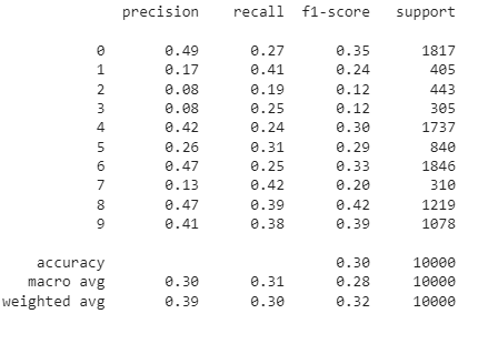
Now, evaluate the model with the test images by obtaining its classification report, confusion matrix, and accuracy score.

accuracy_score(y_pred,y_test)
print(classification_report(y_pred,y_test))

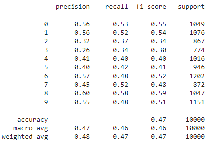
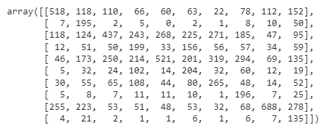
confusion_matrix(y_pred,y_test)

 

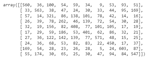
Thus, Random Forest Classifier shows only 47% accuracy on the test set.

Implementing a KNN

KNN stands for K-Nearest neighbours. It is also an algorithm popularly used for multi-class classification.

It is implemented in sklearn using KNeighborsClassifier class. We begin by importing it:

from sklearn.neighbors import KNeighborsClassifier

and then instantiating it to create a KNN model:

knn=KNeighborsClassifier(n_neighbors=7)

I have chosen 7 neighbours randomly. Feel free to play with the number of neighbours to arrive at a better and thus optimal model.

Finally, train it:

knn.fit(x_train2,y_train)

Now, predict for the test set using the fitted KNN model:

y_pred_knn=knn.predict(x_test2)
y_pred_knn

The predictions are outputs representing the classes as described in the previous algorithm.

Now, proceed to evaluate the KNN model just the way we evaluated our previous model.

accuracy_score(y_pred_knn,y_test)
print(classification_report(y_pred_knn,y_test))

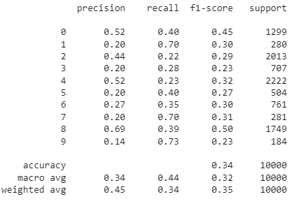
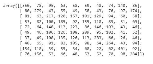
confusion_matrix(y_pred_knn,y_test)

Thus, the KNN Classifier shows only 34% accuracy on the test set.

Implementing a Decision Tree

It is implemented in sklearn using the DecisionTreeClassifier class. We begin by importing it:

from sklearn.tree import DecisionTreeClassifier

and then instantiating it to create a DecisionTreeClassifier model:

dtc=DecisionTreeClassifier()

Finally, train it:

dtc.fit(x_train2,y_train)

Now, predict for the test set using the fitted decision tree model:

y_pred_dtc=dtc.predict(x_test2)

y_pred_dtc

The predictions are outputs representing the classes as described in the previous algorithm.

Now, proceed to evaluate the decision tree model just the way we evaluated our previous model.

accuracy_score(y_pred_dtc,y_test)
print(classification_report(y_pred_dtc,y_test))

confusion_matrix(y_pred_dtc,y_test)

 

Thus, the Decision tree Classifier shows only 27% accuracy on the test set.

Implementing a Naive Bayes classifier

It is the most fundamental machine learning classifier, also abbreviated as NB. It works based on Bayes Theorem and has independent features.

It is implemented in sklearn using the GaussianNB class. We begin by importing it:

from sklearn.naive_bayes import GaussianNB

and then instantiating it to create an NB model:

nb=GaussianNB()

Finally, train it:

nb.fit(x_train2,y_train)

Now, predict for the test set using the fitted NB model:

y_pred_nb=nb.predict(x_test2)

y_pred_nb

The predictions are outputs representing the classes as described in the previous algorithm.

Now, proceed to evaluate the decision tree model just the way we evaluated our previous model.

accuracy_score(y_pred_nb,y_test)
print(classification_report(y_pred_nb,y_test))

confusion_matrix(y_pred_nb,y_test)

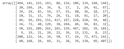
Thus, the Naive Bayes Classifier shows only 30% accuracy on the test set.

Results

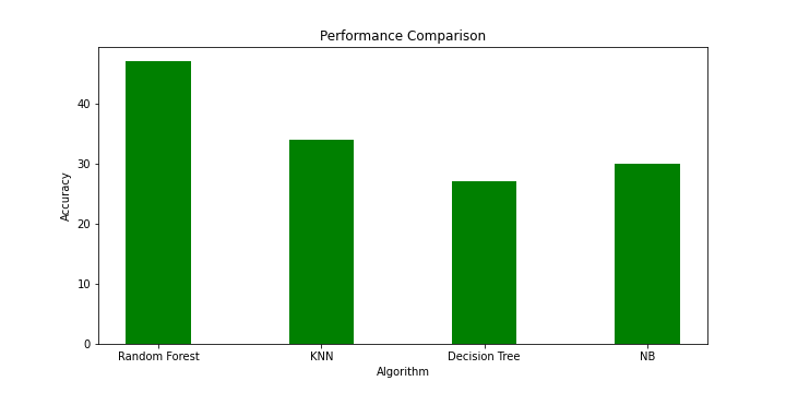
The accuracies of the four ML algorithms, we just explored for our CIFAR-10 dataset, can be summarized using the graph shown above.

Random Forest Classifier shows the best performance with 47% accuracy followed by KNN with 34% accuracy, NB with 30% accuracy, and Decision Tree with 27% accuracy. Thus, Random Forest exhibits the best performance and Decision Tree the worst.

However, all the Machine learning algorithms perform poorly as indicated by the accuracies. The highest is just 47% while Deep learning algorithms outsmart them exceptionally with accuracies mostly exceeding 90%!!!

That’s why I mentioned at the beginning itself that this work can only be used to compare a Deep Learning model and defend the DL model.

Testing for custom input

From the above results, as RandomForestClassifier shows the best performance among all and a decent accuracy as well, let us choose this model.

Custom input refers to a single image that you want to pass to the model and test. Testing a model for a single input is widely used in various real-time applications. For instance, an individual’s photo is inputted into the system for face recognition.

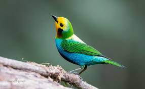
I have used the following custom image to test my model:

                                                                                                       Source

Mention the path of your image-the location where you have stored the custom image you want to test.

img_path='/content/bird.jfif'

NOTE: As I have implemented the work on Google Colab,I uploaded an image there and included the path of the image accordingly.Change the value of img_path according to the location of the image you want to test.

First, read the image using OpenCV and then resize it to 32×32.

img_arr=cv2.imread(img_path)
img_arr=cv2.resize(img_arr,(32,32))

#so,eventually,model.predict() should also be a 2d input
nx, ny, nrgb = img_arr.shape
img_arr2 = img_arr.reshape(1,(nx*ny*nrgb))

classes = ["airplane","automobile","bird","cat","deer","dog","frog","horse","ship","truck"]

ans=model.predict(img_arr2)
print(classes[ans[0]])
#RandomForestClassifier

Conclusion

Thus, in this blog, we discussed how to use image classification in Machine Learning by implementing four common ML algorithms including Random Forest, KNN, Decision Tree, and Naive Bayes classifier. Due to their poor accuracies, Deep learning is preferred for image classification tasks.

You can explore this work further by trying to improve these image classification in ML models using hyperparameter tuning. You may arrive at better accuracies in that case! Go ahead and try!

About Me

I am Nithyashree V, a final year BTech Computer Science and Engineering student. I love learning such cool technologies and putting them into practice, especially observing how they help us solve society’s challenging problems. My areas of interest include Artificial Intelligence, Data Science, and Natural Language Processing.

You can read my other articles on Analytics Vidhya from here.

You can find me on LinkedIn from here.

The media shown in this article is not owned by Analytics Vidhya and are used at the Author’s discretion.