Classifying Sanskrit Shlokas Using an LSTM-based Model

This article was published as a part of the Data Science Blogathon.

Introduction

One isn’t obscure to the kind of knowledge that ancient Indian scriptures treasure. Though these scriptures are in many languages, most of them happen to be in Sanskrit. So, why not employ the power of Natural Language Processing and fiddle a little with Sanskrit text?

Sanskrit is one of the most ancient and unambiguous languages in the world. It is one of the few languages that identifies three grammatical genders (Masculine, Feminine, and Neuter) and three grammatical counting cases (Singular, Plural, and Dual). Given its inclusiveness and unambiguity, a few studies argue that Sanskrit is one of the best-suited languages for Natural Language Processing. Though Sanskrit is not practiced as a modern-day language, its text is available in abundance in Hindu scriptures and ancient Indian literature.

In this article, we will try our hands on NLP in Sanskrit. We will be performing the classification of Sanskrit Shlokas (Verses).

Categorization of Sanskrit Shlokas

First, let us understand what Sanskrit Slokas are and on what grounds we will classify them. So this is how a quick Google search defines the term ‘Shloka’:

Shloka: a couplet of Sanskrit verse, especially one in which each line contains sixteen syllables.

These couplets, written in Sanskrit, usually embody religious praises or knowledge of the ways of life.

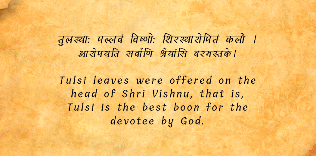
The following is a typical example of a Shloka along with its English translation:

For our classification task, we will be classifying the Shlokas into the following three classes:

1. Chanakya Shlokas: These Shlokas are the ones obtained from The Chanakya Niti Sastra, which is an anthology of Shlokas compiled from various Hindu sastras attributed to the Indian philosopher Chanakya.
2. Vidur Niti Shlokas: These Slokas belong to Vidura Niti, which is an ethical philosophy that was narrated in the form of a conversation, a rich discourse on polity and religiousness between Vidura and King Dhritarashtra in Mahabharata (a Hindu Epic tale)
3. Sanskrit Slogans: These Shlokas are not attributed to any particular source. This can be treated as the ‘others’ category.

Dataset

We will be using the iNLTK Sanskrit Shlokas Dataset that comprises about 500 Shlokas labeled as Chanakya Slokas, Vidur Niti Slokas and Sanskrit-slogan. The Shlokas have already been cleaned and divided into training and testing as CSV files.

The dataset can be obtained from Kaggle. Please note that the dataset lies under the Creative Commons licence.

Building the Shloka Classifier

Let us tackle this stepwise. Firstly, as the classic data science advice says, we should get to know our data better and then build our model accordingly. We’ll proceed in three broad steps:

1. Exploratory Data Analysis
2. Data Pre-Processing
3. Model Building and Evaluation

Exploratory Data Analysis

Step-1: Import all the requisite Python libraries

#Import Necessary Libraries
import pandas as pd
import numpy as np
from wordcloud import WordCloud
import matplotlib.pyplot as plt

Here, we’ve used Pandas to load the CSV dataset, Numpy to perform mathematical operations, word cloud to build a visual of our text and Matplotlib to plot graphs as required.

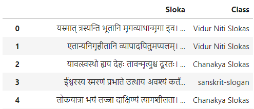
Step-2: Load the Dataset

This is what our data looks like:

#Loading the dataset
data = pd.read_csv('../input/sanskrit-shlokas-dataset/train.csv')

Step-3: Create text Vocabulary-Frequency distribution

Now we need to create a Vocabulary-Frequency distribution for our text. Vocabulary refers to the set of unique words in a text. So we need to store each unique word and its frequency of occurrence in our dataset.

For this, we have first stored all the Shlokas in the training dataset into a single string named ‘text’. Then we stored each unique word as a key in a dictionary named ‘vocab’ and its frequency as the value.

This distribution will help us identify the stopwords in our text. An excerpt from the distribution is shown below:

'पञ्च': 2,

'यत्र': 10,

'न': 122,

'विद्यन्ते': 2,

'कुर्यात्तत्र': 1,

 'संगतिम्': 1,

(The entire distribution is too long to be displayed here)

Step-4: Identify Stopwords from the dataset:

In this step, we’ll identify the stopwords from our dataset. Stopwords are the repeatedly occurring words in a text that usually do not add much value to the meaning or intent of the text. Some examples of stopwords in English are: a, an, the, is, are, have, in, etc. These words occur way too often in the language but do not add to its meaning.

#Generating top 2 percentile list 
freqs = np.array(list(vocab.values()))
percentile_val = np.percentile(freqs, 99)

#Identifying and Storing Stopwords
stopwords = list()
for i in vocab.keys():
    if vocab[i] > percentile_val:
        stopwords.append(i)

To identify stopwords from the text, we just need to pick the most frequently occurring words from the vocabulary. But we need to set a threshold on the frequency of a word for it to qualify as a stopword. In our case, we have set the threshold as 99th percentile i.e. words with a frequency of more than 99 percent of words will be categorized as a stopword. Some of the stopwords obtained are shown below:

['स',
 'यत्र',
 'न',
 'भार्या',
 'सर्वं',
 'हि',
 '।',
 'च',
 '॥न',
 'वै',
 'सर्वत्र',
 'नास्ति',
 'मित्रं',
 'विद्या',
 'एव',
 'तस्य',
 'यो',
 'तु',
 'च।',
 'रक्ष्यते',
 'यः']

Step-5: Plot a Word Cloud of the Text

Now, we will plot a word cloud of the training text. We pass stopwords as a parameter to the word cloud to ensure they are omitted in the output. Besides, since the word cloud, as such, does not support any Sanskrit/Hindi font, one has to download a relevant font and pass its path as a parameter to the word cloud. The font that I used can be found here on Google Fonts.

wordcloud = WordCloud(font_path= '../input/devanagari/TiroDevanagariSanskrit-Regular.ttf',width = 800, height = 800,background_color = 'white', stopwords = stopwords,min_font_size = 10).generate(text)

# plot the WordCloud image
plt.figure(figsize = (8, 8), facecolor = None)
plt.imshow(wordcloud)
plt.axis('off')

The generated word cloud looks like this:

Step-6: Plot the Output class label frequencies

Now, we’ll generate a bar chart for the frequencies of each output class label.

#Plot class label frequencies
Class = data['Class'].value_counts()
names = ['Chanakya Slokas','Vidur Niti Slokas','sanskrit-slogan']
values = [Class['Chanakya Slokas'],Class['Vidur Niti Slokas'],Class['sanskrit-slogan']]

plt.bar(range(len(values)), values, tick_label=names)
plt.show()

The bar chart turns out as follows:

We can see that number of training examples corresponding to each class is nearly equal i.e. our dataset is balanced.

By now, we have gained quite decent insight into our data; now, let’s move on to pre-processing the data.

Data Pre-Processing

Since we’ll be building an LSTM-based deep learning classifier, we first need to convert our training text into embeddings. For this, we’ll use TensorFlow’s tokenizer. First, we need to train the tokenizer on the entire training text to ensure it fits on its vocabulary. Then we convert the training text to embeddings using the texts_to_sequences() method. Finally, we pad all the generated sequences so as to make them equal in length.

from keras.preprocessing.text import Tokenizer
from keras.preprocessing.sequence import pad_sequences

tokenizer = Tokenizer(num_words=500, split=' ') 
tokenizer.fit_on_texts(data['Sloka'].values)
X = tokenizer.texts_to_sequences(data['Sloka'].values)
X = pad_sequences(X)

The generated embeddings would look like this:

array([[  0,   0,   0, ...,   6, 320,   1],
       [  0,   0,   0, ..., 326, 327,   1],
       [  0,   0,   0, ..., 334,  19, 335],
       ...,
       [  0,   0,   0, ..., 239,  76,  42],
       [  0,   0,   0, ...,   4, 100,  38],
       [  0,   0,   0, ...,   0,   0,   1]], dtype=int32)

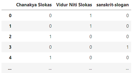
After generating the embeddings, our text is ready to be fed to any model. But we must note that our output classes are categorical in nature. Thus, they must be one hot encodes. You can use sklearn’s one hot encoder for the same. However, here I’ve used Pandas’ get_dummies function.

#One Hot Encoding 
Y= pd.get_dummies(data['Class'])

The One Hot Encoded Vector (Y) looks like this:

 

Model Building and Evaluation

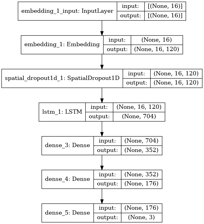
Now that our data is ready and waiting to be fed to some model, let us get on to building one. Since we are dealing with a text classification use case, we’ll go ahead with an LSTM-based model. LSTMs (Long Short Term Memory) combines the capabilities of RNNs (Recurrent Neural Networks) with the advantages of memory units that make them suitable for NLP tasks. If you’d like to learn about LSTMs in great detail, I’d recommend you go through this article.

#Model Building
model = Sequential()
model.add(Embedding(500, 120, input_length = X.shape[1]))
model.add(SpatialDropout1D(0.4))
model.add(LSTM(704, dropout=0.4, recurrent_dropout=0.4))
model.add(Dense(352, activation='LeakyReLU'))
model.add(Dense(176, activation='LeakyReLU'))
model.add(Dense(3,activation='softmax'))
model.compile(loss = 'categorical_crossentropy', optimizer='adam', metrics = ['accuracy'])
print(model.summary())

The model summary is as follows:

Model: "sequential_1"
_________________________________________________________________
Layer (type)                 Output Shape              Param #   
=================================================================
embedding_1 (Embedding)      (None, 16, 120)           60000     
_________________________________________________________________
spatial_dropout1d_1 (Spatial (None, 16, 120)           0         
_________________________________________________________________
lstm_1 (LSTM)                (None, 704)               2323200   
_________________________________________________________________
dense_3 (Dense)              (None, 352)               248160    
_________________________________________________________________
dense_4 (Dense)              (None, 176)               62128     
_________________________________________________________________
dense_5 (Dense)              (None, 3)                 531       
=================================================================
Total params: 2,694,019
Trainable params: 2,694,019
Non-trainable params: 0
_________________________________________________________________

The layer-by-layer description of the model can be seen below:

Please note that since ours is a case of multi-class classification (i.e., we are classifying our input text into more than two classes), thus we have used ‘softmax’ as the activation function in the output layer and ‘categorical_corssentropy’ as the loss function.

Now, we will fit the model into our training data.

history  = model.fit(X, Y, epochs = 30, batch_size=32, verbose =1)

The training accuracy turns out to be 94.34% in this case.

Now, to test our model on new data, we need to prepare/pre-process our test data, just as we did with our training data.

#Loading the test data
test = pd.read_csv('../input/sanskrit-shlokas-dataset/valid.csv')

#Tokenize the input texts
X_test = tokenizer.texts_to_sequences(test['Sloka'].values)
X_test = pad_sequences(X_test)

#One Hot Encode the Output Classes
Y_test = pd.get_dummies(test['Class'])

So, we have loaded our test data, tokenized its input text, and one hot encoded its output classes. Thus, our test data is ready for model evaluation!

model.evaluate(X_test,Y_test)

Finally, we have obtained a test accuracy of 78%, which is quite decent.

What’s Next?

You’ve finally built a Sanskrit Shloka Classification model using LSTM from scratch. Give yourself a pat on the back! Though this was a small dataset, you can try finding new datasets or perhaps create one on your own to ensure a more robust model.

Here’s a quick recap of what this article encompasses:

• We have successfully classified shlokas into three categories: Chanakya Shlokas, Vidhur Niti Shlokas, and Sanskrit Slogans.
• We also learned how to extract stopwords from the language using a vocabulary-frequency distribution and visualize text using word clouds.
• Finally, we built an LSTM model using TensorFlow and tuned its parameters to perform the multi-class classification task.

That’s all for this article; feel free to leave a comment with any feedback or questions.

Since you’ve read the article up till here, I’m certain our interests do match — so please feel to connect with me on LinkedIn or Instagram for any queries or potential opportunity

The media shown in this article is not owned by Analytics Vidhya and is used at the Author’s discretion.