Calibration of Machine Learning Models
This article was published as a part of the Data Science Blogathon.
Introduction

A screen image related to a weather forecast must be a familiar picture to most of us. The AI Model predicting the expected weather predicts a 40% chance of rain today, a 50% chance of Wednesday, and a 50% on Thursday. Here the AI/ML Model is talking about the probability of occurrence, which is the interesting part. Now, the question is this AI/ML model trustworthy?
As learners of Data Science/Machine Learning, we would have walked through stages where we build various supervisory ML Models(both classification and regression models). We also look at different model parameters that tell us how well the model performs. One important but probably not so well-understood model reliability parameter is Model Calibration. The calibration tells us how much we can trust a model prediction. This article explores the basics of model calibration and its relevancy in the MLOps cycle. Even though Model Calibration applies to regression models as well, we will exclusively look at classification examples to get a grasp on the basics.
The Need for Model Calibration
Wikipedia amplifies calibration as ” In measurement technology and metrology, calibration is the comparison of measurement values delivered by a device under test with those of a calibration standard of known accuracy. “
The model outputs two important pieces of information in a typical classification ML model. One is the predicted class label (for example, classification as spam or not spam emails), and the other is the predicted probability. In binary classification, the sci-kit learn library gives a method called the model.predict_proba(test_data) that gives us the probability for the target to be 0 and 1 in an array form. A model predicting rain can give us a 40% probability of rain and a 60% probability of no rain. We are interested in the uncertainty in the estimate of a classifier. There are typical use cases where the predicted probability of the model is very much of interest to us, such as weather models, fraud detection models, customer churn models, etc. For example, we may be interested in answering the question, what is the probability of this customer repaying the loan?
Let’s say we have an ML model which predicts whether a patient has cancer-based on certain features. The model predicts a particular patient does not have cancer (Good, a happy scenario!). But if the predicted probability is 40%, then the Doctor may like to conduct some more tests for a certain conclusion. This is a typical scenario where the prediction probability is critical and of immense interest to us. The Model Calibration helps us improve the model’s prediction probability so that the model’s reliability improves. It also helps us to decipher the predicted probability observed from the model predictions. We can’t take for granted that the model is twice as confident when giving a predicted probability of 0.8 against a figure of 0.4.
We also must understand that calibration differs from the model’s accuracy. The model accuracy is defined as the number of correct predictions divided by the total number of predictions made by the model. It is to be clearly understood that we can have an accurate but not calibrated model and vice versa.
If we have a model predicting rain with 80% predicted probability at all times, then if we take data for 100 days and find 80 days are rainy, we can say that model is well calibrated. In other words, calibration attempts to remove bias in the predicted probability.
Consider a scenario where the ML model predicts whether the user who is making a purchase on an e-commerce website will buy another associated item or not. The model predicts the user has a probability of 68% for buying Item A and an item B probability of 73%. Here we will present Item B to the user(higher predicted probability), and we are not interested in actual figures. In this scenario, we may not insist on strict calibration as it is not so critical to the application.
The following shows details of 3 classifiers (assume that models predict whether an image is a dog image or not). Which of the following model is calibrated and hence reliable?
(a) Model 1 : 90% Accuracy, 0.85 confidence in each prediction
(b) Model 2 : 90% Accuracy, 0.98 confidence in each prediction
(c) Model 3 : 90% Accuracy ,0.91 confidence in each prediction
If we look at the first model, it is underconfident in its prediction, whereas model 2 seems overconfident. Model 3 seems well-calibrated, giving us confidence in the model’s ability. Model 3 thinks it is correct 91% of the time and 90% of the time, which shows good calibration.
Reliability Curves
The model’s calibration can be checked by creating a calibration plot or Reliability Plot. The calibration plot reveals the disparity between the probability predicted by the model and the true class probabilities in the data. If the model is well calibrated, we expect to see a straight line at 45 degrees from the origin (indicative that estimated probability is always the same as empirical probability ).
We will attempt to understand the calibration plot using a toy dataset to concretize our understanding of the subject.
The following data contains the predicted probability of a model and True y values. It is easier to handle the data when sorted in terms of probability.
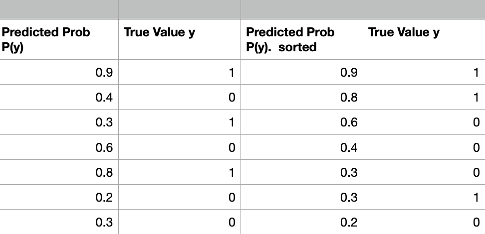
The resulting probability is divided into multiple bins representing possible ranges of outcomes. For example, [0-0.1), [0.1-0.2), etc., can be created with 10 bins. For each bin, we calculate the percentage of positive samples. For a well-calibrated model, we expect the percentage to correspond to the bin center. If we take the bin with the interval [0.9-1.0), the bin center is 0.95, and for a well-calibrated model, we expect the percentage of positive samples ( samples with label 1) to be 95%.
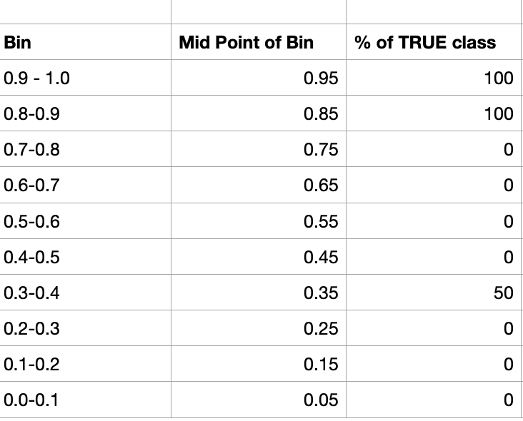
We can plot the Mean predicted value (midpoint of the bin ) vs. Fraction of TRUE Positives in each bin in a line plot to check the calibration. of the model.
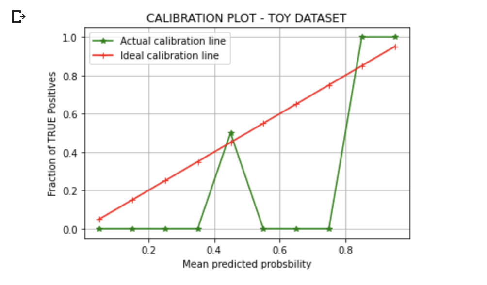
We can see the difference between the ideal curve and the actual curve, indicating the need for our model to be calibrated. Suppose the points obtained are below the diagonal. In that case, it indicates that the model has overestimated (model predicted probabilities are too high). If the points are above the diagonal, it can be estimated that model has been underconfident in its predictions(the probability is too small). Let’s also look at a real-life Random Forest Model curve in the image below.
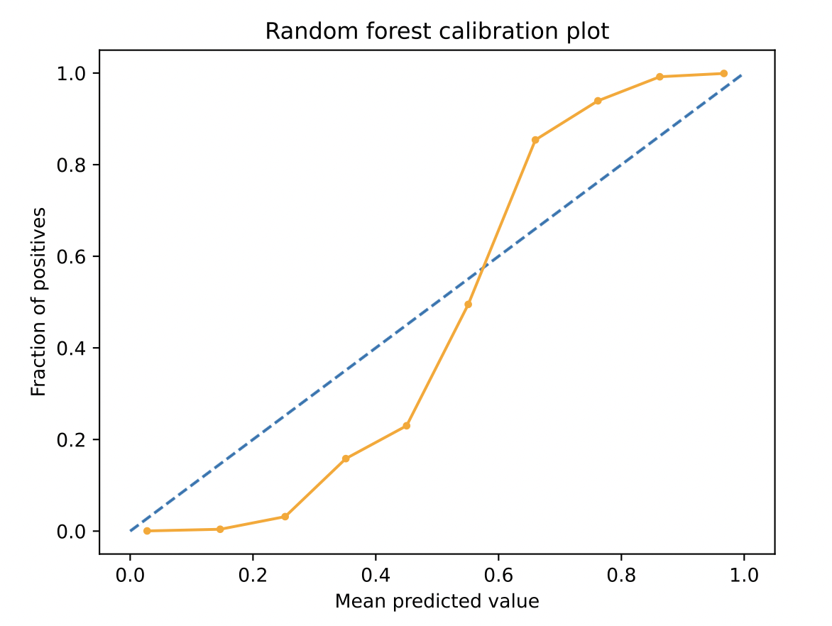
If we look at the above plot, the S curve ( remember the sigmoid curve seen in Logistic Regression !) is observed commonly for some models. The Model is seen to be underconfident at high probabilities and overconfident when predicting low probabilities. For the above curve, for the samples for which the model predicted probability is 30%, the actual value is only 10%. So the Model was overestimating at low probabilities.
The toy dataset we have shown above is for understanding, and in reality, the choice of bin size is dependent on the amount of data we have, and we would like to have enough points in each bin such that the standard error on the mean of each bin is small.
Brier Score
We do not need to go for the visual information to estimate the Model calibration. The calibration can be measured using the Brier Score. The Brier score is similar to the Mean Squared Error but used slightly in a different context. It takes values from 0 to 1, with 0 meaning perfect calibration, and the lower the Brier Score, the better the model calibration.
The Brier score is a statistical metric used to measure probabilistic forecasts’ accuracy. It is mostly used for binary classification.
Let’s say a probabilistic model predicts a 90% chance of rain on a particular day, and it indeed rains on that day. The Brier score can be calculated using the following formula,
Brier Score = (forecast-outcome)2
Brier Score in the above case is calculated to be (0.90-1)2 = 0.01.
The Brier Score for a set of observations is the average of individual Brier Scores.
On the other hand, if a model predicts with a 97% probability that it will rain but does not rain, then the calculated Brier Score, in this case, will be,
Brier Score = (0.97-0)2 = 0.9409 . A lower Brier Score is preferable.
Calibration Process
Now, let’s try and get a glimpse of how the calibration process works without getting into too many details.
Some algorithms, like Logistic Regression, show good inherent calibration standards, and these models may not require calibration. On the other hand, models like SVM, Decision Trees, etc., may benefit from calibration. The calibration is a rescaling process after a model has made the predictions.
There are two popular methods for calibrating probabilities of ML models, viz,
(a) Platt Scaling
(b) Isotonic Regression
It is not the intention of this article to get into details of the mathematics behind the implementation of the above approaches. However, let’s look at both methods from a ringside perspective.
The Platt Scaling is used for small datasets with a reliability curve in the sigmoid shape. It can be loosely understood as putting a sigmoid curve on top of the calibration plot to modify the predictive probabilities of the model.
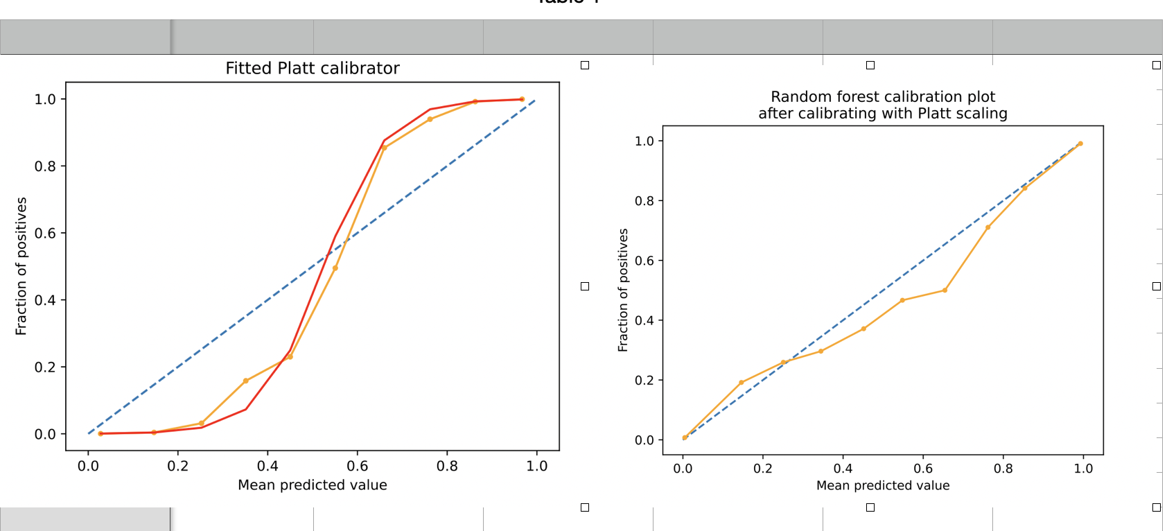
The above images show how imposing a Platt calibrator curve on the reliability curve of the model modifies the curve. It is seen that the points in the calibration curve are pulled toward the ideal line (dotted line) during the calibration process.
Isotonic Regression is a more complex approach and requires more data. The main advantage of Isotonic Regression is that it doesn’t require the reliability curve of the model to be S-shaped. However, this method is sensitive to outliers and works well for large datasets.
It is noted that for practical implementation during model development, standard libraries like sklearn support easy model calibration(sklearn.calibration.CalibratedClassifier).
Impact on Performance
It is pertinent to note that calibration modifies the outputs of trained ML models. It could be possible that calibration also affects the model’s accuracy. Post calibration, some values close to the decision boundary (say 50% for binary classification) may be modified in such a way as to produce an output label different from prior calibration. The impact on accuracy is rarely huge, and it is important to note that calibration improves the reliability of the ML model.
Conclusion
In this article, we have looked at the theoretical background of Model Calibration. Calibration of Machine Learning models is an important but often overlooked aspect of developing a reliable model. The following are key takeaways from our learnings:-
(a) Model Calibration gives insight or understanding of uncertainty in the prediction of the model and in turn, the reliability of the model to be understood by the end-user, especially in critical applications.
(b) Model calibration is extremely valuable to us in cases where predicted probability is of interest.
(c) Reliability curves and Brier Score gives us an estimate of the calibration levels of the model.
(c) Platt scaling and Isotonic Regression is popular methods to scale the calibration levels and improve the predicted probability.
Where do we go from here? This article aims to give you a basic understanding of Model Calibration. We can further build on this by exploring actual implementation using standard python libraries like scikit Learn for use cases.
The media shown in this article is not owned by Analytics Vidhya and is used at the Author’s discretion.


