Deep learning model to predict mRNA Degradation
This article was published as a part of the Data Science Blogathon
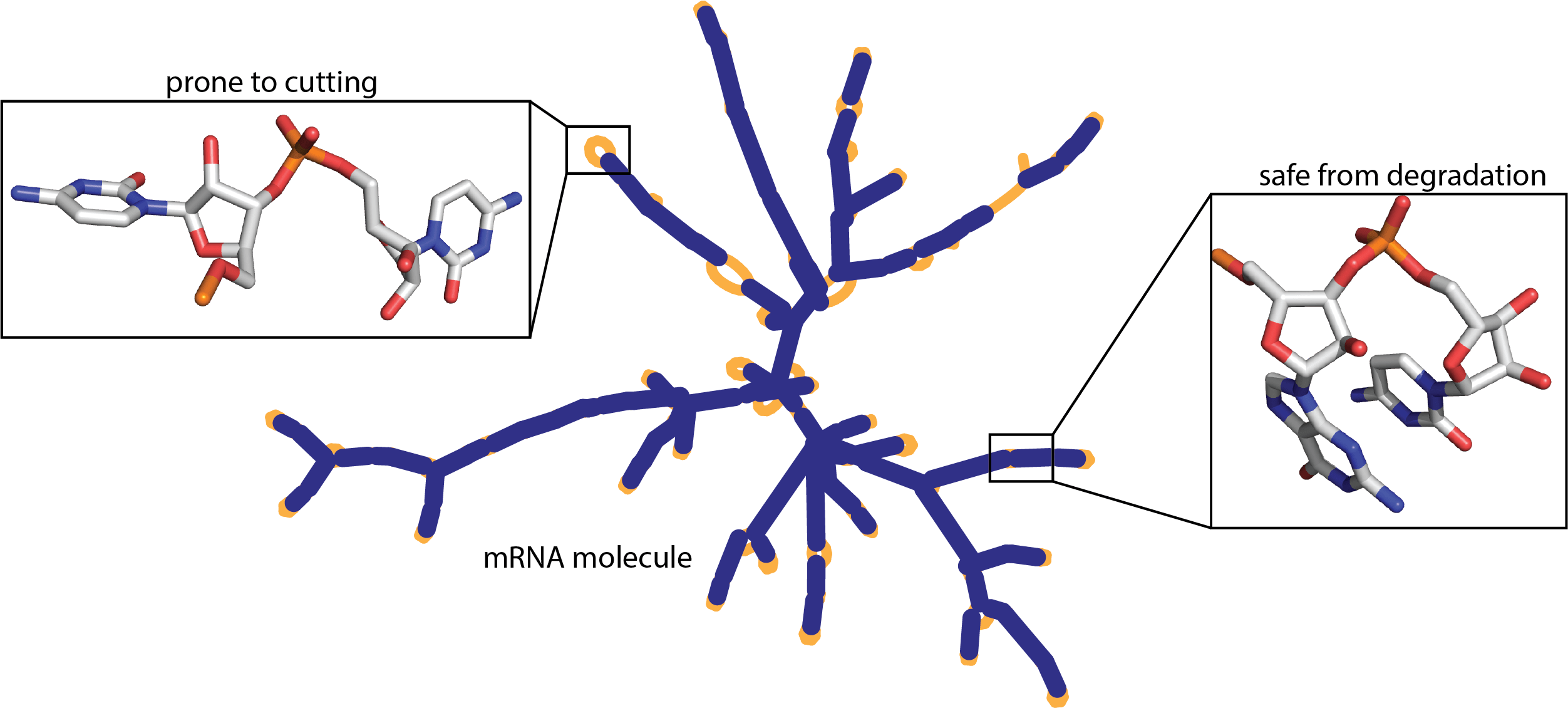
Designing a deep learning model that will predict degradation rates at each base of an RNA molecule using the Eterna dataset comprising over 3000 RNA molecules.

Introduction
Project Objectives
In this project, we are going to use explore our dataset and then preprocessed sequence, structure, and predicted loop type features so that they can be used to train our deep learning GRU model. Finally predicting degradation records on public and test datasets.
Importing the Libraries necessary to Predict mRNA Degradation
We will be using TensorFlow as our main library to build and train our model and JSON/Pandas to ingest the data. For visualization, we are going to use Plotly and for data manipulation Numpy.
# Dataframe
import json
import pandas as pd
import numpy as np
# Visualization
import plotly.express as px
# Deeplearning
import tensorflow.keras.layers as L
import tensorflow as tf
# Sklearn
from sklearn.model_selection import train_test_split
#Setting seeds
tf.random.set_seed(2021)
np.random.seed(2021)
Training Parameters
- Target columns: reactivity, deg_Mg_pH10, deg_Mg_50C, deg_pH10, deg_50C
- Model_Train: True if you want to Train a model which takes 1 hour to train.
# This will tell us the columns we are predicting
target_cols = ['reactivity', 'deg_Mg_pH10', 'deg_Mg_50C', 'deg_pH10', 'deg_50C']
Model_Train = True # True if you want to Train model which take 1 hour to train.
Metric to Evaluate the mRNA Degradation Prediction
Our model performance metric is MCRMSE (Mean column-wise root mean squared error), which takes root mean square error of ground truth of all target columns.

where is the number of scored ground truth target columns, and are the actual and predicted values, respectively?
def MCRMSE(y_true, y_pred):## Monte Carlo root mean squared errors
    colwise_mse = tf.reduce_mean(tf.square(y_true - y_pred), axis=1)
    return tf.reduce_mean(tf.sqrt(colwise_mse), axis=1)
Loading Data
The mRNA degradation data is available on Kaggle.
Detailed Explanation of the Data
- id – Unique identifier sample.
- seq_scored – This should match the length of reactivity, deg_*, and error columns.
- seq_length – The length of the sequence.
- sequence – Describes the RNA sequence, a combination of A, G, U, and C for each sample.
- structure – An array of (, ), and. characters donate to the base is to be paired or unpaired.
- reactivity – These numbers are reactivity values for the first 68 bases used to determine the likely secondary structure of the RNA sample.
- deg_pH10 – The likelihood of degradation after incubating without magnesium on pH10 at base or linkage.
- deg_Mg_pH10 – The likelihood of degradation after incubating with magnesium on pH 10 at base or linkage.
- deg_50C – The likelihood of degradation after incubating without magnesium at 50 degrees Celsius at base or linkage.
- deg_Mg_50C – The likelihood of degradation after incubating with magnesium at 50 degrees Celsius at base or linkage.
- *_error_* – calculated errors in experimental values obtained in reactivity, and deg_* columns.
- predicted_loop_type – Loop types assigned by bpRNA from Vienna which suggests:
- S: paired Stem
- M: Multiloop
- I: Internal loop
- B: Bulge
- H: Hairpin loop
- E: dangling End
- X: external loop
Observing Data
data_dir = "stanford-covid-vaccine/"
train = pd.read_json(data_dir + "train.json", lines=True)
test = pd.read_json(data_dir + "test.json", lines=True)
sample_df = pd.read_csv(data_dir + "sample_submission.csv")
we have sequence, structure, and predicted loop types that are in text formats. We will be converting them into numerical tokens so that they can be used to train deep learning models. Then we have arrays within columns from reactivity_error to deg_50C that we will be using as targets.
train.head(2)
print('Train shapes: ', train.shape) print('Test shapes: ', test.shape)
Train shapes:  (2400, 19)
Test shapes:  (3634, 7)
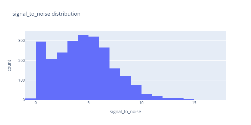
Signal to noise distribution in mRNA Degradation Prediction Data
We can see the signal-to-noise distribution is between 0 to 15 and the majority of samples lie between 0-6. We have also negative values that we need to get rid of.
fig = px.histogram(
    train,
    "signal_to_noise",
    nbins=25,
    title='signal_to_noise distribution',
    width=800,
    height=400
)
fig.show()
Removing negative values
train = train.query("signal_to_noise >= 1")
Sequence Test length
After looking at sequence length distribution we know that we have two distinctive sequence lengths, one at 107 and another at 130.
fig = px.histogram(
    test,
    "seq_length",
    nbins=25,
    title='sequence_length distribution',
    width=800,
    height=400
)
fig.show()
.png)
Splitting Test into Public and Private DataFrame
Let’s split our test dataset based on sequence length. Doing this will improve the overall performance of our GRU model.
public_df = test.query("seq_length == 107")
private_df = test.query("seq_length == 130")
Pre-processing Data
token2int = {x: i for i, x in enumerate("().ACGUBEHIMSX")}
token2int
{'(': 0,
 ')': 1,
 '.': 2,
 'A': 3,
 'C': 4,
 'G': 5,
 'U': 6,
 'B': 7,
 'E': 8,
 'H': 9,
 'I': 10,
 'M': 11,
 'S': 12,
 'X': 13}
Converting DataFrame to 3D Array
The function below takes a Pandas data frame and converts it into a 3D NumPy array. We will be using it to convert both training features and targets.
def dataframe_to_array(df):
   return np.transpose(np.array(df.values.tolist()), (0, 2, 1))
Tokenization of Sequence
The function below uses a string to integer dictionary that we had created early to convert training features into arrays containing integers. Then we will be using dataframe_to_array to convert our dataset into a 3D NumPy array.
def dataframe_label_encoding(
    df, token2int, cols=["sequence", "structure", "predicted_loop_type"]
):
    return dataframe_to_array(
        df[cols].applymap(lambda seq: [token2int[x] for x in seq])
    ) ## tokenization of Sequence, Structure, Predicted loop
Preprocessing Features and Labels
- Using label endorsing function on our training features.
- Converting target data frame into a 3D array.
train_inputs = dataframe_label_encoding(train, token2int) ## Label encoding
train_labels = dataframe_to_array(train[target_cols]) ## dataframe to 3D array to
Train & Validation split
Splitting our training data into train and validation sets. We are using signal to noise filter to equally distribute our dataset.
x_train, x_val, y_train, y_val = train_test_split(
    train_inputs, train_labels, test_size=0.1, random_state=34, stratify=train.SN_filter
)
Preprocessing Public and Private Dataframe
Earlier we have split our test dataset into public and private based on sequence length now we are going to use dataframe_label_encoding to tokenized and reshape it into NumPy array as we have done the same with the training dataset.
public_inputs = dataframe_label_encoding(public_df, token2int)
private_inputs = dataframe_label_encoding(private_df, token2int)
Training / Evaluating the mRNA Degradation Prediction Model
Build Model
Before jumping directly into the deep learning model, we have tested other gradient boosts such as Light GBM and CatBoost. Then as we were dealing with the sequence, I thought to experiment around BiLSTM model, but they all performed worst compared to the triple GRU model with linear activation.
This model is influenced by xhlulu initial models. I amazed me how simple the GRU layer can produce the best results possible without using data augmentation or feature engineering.
To learn more about RNNs, LSTM and GRU, please see this blog post.
def build_model(
    embed_size, # Length of unique tokens
    seq_len=107, # public dataset seq_len
    pred_len=68, # pred_len for public data
    dropout=0.5, # trying best dropout (general)
    sp_dropout=0.2, # Spatial Dropout
    embed_dim=200, # embedding dimension
    hidden_dim=256, # hidden layer units
):
    inputs = L.Input(shape=(seq_len, 3))
    embed = L.Embedding(input_dim=embed_size, output_dim=embed_dim)(inputs)
    reshaped = tf.reshape(
        embed, shape=(-1, embed.shape[1], embed.shape[2] * embed.shape[3])
    )
    hidden = L.SpatialDropout1D(sp_dropout)(reshaped)
     # 3X BiGRU layers
    hidden = L.Bidirectional(
        L.GRU(
            hidden_dim,
            dropout=dropout,
            return_sequences=True,
            kernel_initializer="orthogonal",
        )
    )(hidden)
    hidden = L.Bidirectional(
        L.GRU(
            hidden_dim,
            dropout=dropout,
            return_sequences=True,
            kernel_initializer="orthogonal",
        )
    )(hidden)
    hidden = L.Bidirectional(
        L.GRU(
            hidden_dim,
            dropout=dropout,
            return_sequences=True,
            kernel_initializer="orthogonal",
        )
    )(hidden)
    # Since we are only making predictions on the first part of each sequence,
    # we have to truncate it
    truncated = hidden[:, :pred_len]
    out = L.Dense(5, activation="linear")(truncated)
    model = tf.keras.Model(inputs=inputs, outputs=out)
    model.compile(optimizer="Adam", loss=MCRMSE) # loss function as of Eval Metric
    return model
Building model to predict mRNA Degradation Prediction
building our model by adding embed size (14) and we are going to use default values for other parameters.
- sequence length: 107
- prediction length: 68
- dropout: 0.5
- spatial dropout: 0.2
- embedded dimensions: 200
- hidden layers dimensions: 256
model = build_model(
    embed_size=len(token2int) ## embed_size = 14
)  ## uniquie token in sequence, structure, predicted_loop_type
model.summary()
Model: "model"
_________________________________________________________________
Layer (type)                 Output Shape              Param #
=================================================================
input_1 (InputLayer)         [(None, 107, 3)]          0
_________________________________________________________________
embedding (Embedding)        (None, 107, 3, 200)       2800
_________________________________________________________________
tf.reshape (TFOpLambda)      (None, 107, 600)          0
_________________________________________________________________
spatial_dropout1d (SpatialDr (None, 107, 600)          0
_________________________________________________________________
bidirectional (Bidirectional (None, 107, 512)          1317888
_________________________________________________________________
bidirectional_1 (Bidirection (None, 107, 512)          1182720
_________________________________________________________________
bidirectional_2 (Bidirection (None, 107, 512)          1182720
_________________________________________________________________
tf.__operators__.getitem (Sl (None, 68, 512)           0
_________________________________________________________________
dense (Dense)                (None, 68, 5)             2565
=================================================================
Total params: 3,688,693
Trainable params: 3,688,693
Non-trainable params: 0
_________________________________________________________________
Training the mRNA Degradation Prediction Model
We are going to train our model for 40 epochs and save the model checkpoint in the Model folder. We have experimented with batch sizes from 16, 32, 64 and by far 64 batch sizes produced better results and fast convergence.
As we can observe both training and validation loss (MCRMSE) is reducing with every iteration until 20 epochs and from there they start to diverge. For the next experimentation, we will be keeping the number of epochs limited to twenty to get fast and better results.
if Model_Train:
    history = model.fit(
        x_train,
        y_train,
        validation_data=(x_val, y_val),
        batch_size=64,
        epochs=40,
        verbose=2,
        callbacks=[
            tf.keras.callbacks.ReduceLROnPlateau(patience=5),
            tf.keras.callbacks.ModelCheckpoint("Model/model.h5"),
        ],
    )
Epoch 1/40
30/30 - 69s - loss: 0.4536 - val_loss: 0.3796
Epoch 2/40
30/30 - 57s - loss: 0.3856 - val_loss: 0.3601
Epoch 3/40
30/30 - 57s - loss: 0.3637 - val_loss: 0.3410
Epoch 4/40
30/30 - 57s - loss: 0.3488 - val_loss: 0.3255
Epoch 5/40
30/30 - 57s - loss: 0.3357 - val_loss: 0.3188
Epoch 6/40
30/30 - 57s - loss: 0.3295 - val_loss: 0.3163
Epoch 7/40
30/30 - 57s - loss: 0.3200 - val_loss: 0.3098
Epoch 8/40
30/30 - 57s - loss: 0.3117 - val_loss: 0.2997
Epoch 9/40
30/30 - 57s - loss: 0.3046 - val_loss: 0.2899
Epoch 10/40
30/30 - 57s - loss: 0.2993 - val_loss: 0.2875
Epoch 11/40
30/30 - 57s - loss: 0.2919 - val_loss: 0.2786
Epoch 12/40
30/30 - 57s - loss: 0.2830 - val_loss: 0.2711
Epoch 13/40
30/30 - 57s - loss: 0.2777 - val_loss: 0.2710
Epoch 14/40
30/30 - 57s - loss: 0.2712 - val_loss: 0.2584
Epoch 15/40
30/30 - 57s - loss: 0.2640 - val_loss: 0.2580
Epoch 16/40
30/30 - 57s - loss: 0.2592 - val_loss: 0.2518
Epoch 17/40
30/30 - 57s - loss: 0.2540 - val_loss: 0.2512
Epoch 18/40
30/30 - 57s - loss: 0.2514 - val_loss: 0.2461
Epoch 19/40
30/30 - 57s - loss: 0.2485 - val_loss: 0.2492
Epoch 20/40
30/30 - 57s - loss: 0.2453 - val_loss: 0.2434
Epoch 21/40
30/30 - 57s - loss: 0.2424 - val_loss: 0.2411
Epoch 22/40
30/30 - 57s - loss: 0.2397 - val_loss: 0.2391
Epoch 23/40
30/30 - 57s - loss: 0.2380 - val_loss: 0.2412
Epoch 24/40
30/30 - 57s - loss: 0.2357 - val_loss: 0.2432
Epoch 25/40
30/30 - 57s - loss: 0.2330 - val_loss: 0.2384
Epoch 26/40
30/30 - 57s - loss: 0.2316 - val_loss: 0.2364
Epoch 27/40
30/30 - 57s - loss: 0.2306 - val_loss: 0.2397
Epoch 28/40
30/30 - 57s - loss: 0.2282 - val_loss: 0.2343
Epoch 29/40
30/30 - 57s - loss: 0.2242 - val_loss: 0.2392
Epoch 30/40
30/30 - 57s - loss: 0.2232 - val_loss: 0.2326
Epoch 31/40
30/30 - 57s - loss: 0.2207 - val_loss: 0.2318
Epoch 32/40
30/30 - 57s - loss: 0.2192 - val_loss: 0.2339
Epoch 33/40
30/30 - 57s - loss: 0.2175 - val_loss: 0.2287
Epoch 34/40
30/30 - 57s - loss: 0.2160 - val_loss: 0.2310
Epoch 35/40
30/30 - 57s - loss: 0.2137 - val_loss: 0.2299
Epoch 36/40
30/30 - 57s - loss: 0.2119 - val_loss: 0.2288
Epoch 37/40
30/30 - 57s - loss: 0.2101 - val_loss: 0.2271
Epoch 38/40
30/30 - 57s - loss: 0.2088 - val_loss: 0.2274
Epoch 39/40
30/30 - 57s - loss: 0.2082 - val_loss: 0.2265
Epoch 40/40
30/30 - 57s - loss: 0.2064 - val_loss: 0.2276
Evaluate training history
Both validation and training loss were reduced until 20 epochs. The validation loss became flat after 35 so in my opinion, we should test results on both 20 and 35 epochs.
if Model_Train:
    fig = px.line(
        history.history,
        y=["loss", "val_loss"],
        labels={"index": "epoch", "value": "MCRMSE"},
        title="History",
    )
    fig.show()
.png)
Loading models and making predictions
The test dataset was divided into public and private sets that have different sequence lengths, so in order to predict degradation on different lengths, we need to build 2 different models and load our saved checkpoints. This is possible because RNN models can accept sequences of varying lengths as inputs. Artificial Intelligence(https://ai.stackexchange.com/questions/2008/how-can-neural-networks-deal-with-varying-input-sizes)
Loading weights
model_public = build_model(seq_len=107, pred_len=107, embed_size=len(token2int))
model_private = build_model(seq_len=130, pred_len=130, embed_size=len(token2int))
model_public.load_weights("Model/model.h5")
model_private.load_weights("Model/model.h5")
Prediction
We have successfully predicted for both public and private data sets. In the next step, we will be combining them using test id.
public_preds = model_public.predict(public_inputs)
private_preds = model_private.predict(private_inputs)
private_preds.shape
(3005, 130, 5)
Post-processing and submit
- combining both private (df,prediction ) and public(df,prediction) data frame.
- Adding series of integers in front of id based on a sequence of single prediction for example
[id_00073f8be_0,id_00073f8be_1,id_00073f8be_2 ..] - Concatenating all of the data into Pandas Dataframe and preparing for submission.
preds_ls = []
for df, preds in [(public_df, public_preds), (private_df, private_preds)]:
    for i, uid in enumerate(df.id):
        single_pred = preds[i]
        single_df = pd.DataFrame(single_pred, columns=target_cols)
        single_df["id_seqpos"] = [f"{uid}_{x}" for x in range(single_df.shape[0])]
        preds_ls.append(single_df)
preds_df = pd.concat(preds_ls)
preds_df.head()
         reactivity	deg_Mg_pH10	deg_Mg_50C	deg_pH10	deg_50C	        id_seqpos
0	0.685760	0.703746	0.585288	1.857178	0.808561	id_00073f8be_0
1	2.158555	3.243329	3.443042	4.394709	3.012130	id_00073f8be_1
2	1.432280	0.674404	0.672512	0.662341	0.718279	id_00073f8be_2
3	1.296234	1.306208	1.898748	1.324560	1.827133	id_00073f8be_3
4	0.851104	0.670810	0.971952	0.573919	0.962205	id_00073f8be_4
Submission
Merging sample data frame with predicted on id_seqpos to avoid repetition and make sure it follows submission format. Finally, save our data frame into .csv file.
submission = sample_df[["id_seqpos"]].merge(preds_df, on=["id_seqpos"])
submission.to_csv("Submission/submission.csv", index=False)
submission.head()
         id_seqpos	reactivity	deg_Mg_pH10	deg_Mg_50C	deg_pH10	deg_50C
0	id_00073f8be_0	0.685760	0.703746	0.585288	1.857178	0.808561
1	id_00073f8be_1	2.158555	3.243329	3.443042	4.394709	3.012130
2	id_00073f8be_2	1.432280	0.674404	0.672512	0.662341	0.718279
3	id_00073f8be_3	1.296234	1.306208	1.898748	1.324560	1.827133
4	id_00073f8be_4	0.851104	0.670810	0.971952	0.573919	0.962205
Private Score
After submission into OpenVaccine: COVID-19 mRNA Vaccine Degradation Prediction | Kaggle we got a private score of 0.2723 which is quite better. This result was produced on 50 epochs as I was trying different parameters to improve my score.
.png)
Conclusion
This was a unique experience for me as I was dealing with JSON files with multiple arrays within single samples. After figuring out how to use that data the challenge became quite simple and the Kaggle community have a bigger part in helping me solve this problem. This article was purely model-based and apart from it I have explored the dataset and used data analysis to make sense of some of the common patterns. I wanted to include my experiments with other gradient boosting and LSTM models, but I wanted to present the best possible model.
We have used JSON files and converted them into tokenized 3D Numpy arrays and then used the 3X GRU model. Finally, we have used saved weights to create distinct models for varying lengths of the RNA sequence. I will suggest you use my code and play around to check whether you can beat my score on the leader board.
Source Code
You can find the source code on dagshub and Deepnote Project.
Additional Data
How RNA vaccines work, and their issues: https://www.pbs.org/wgbh/nova/video/rna-coronavirus-vaccine/
Launch of the OpenVaccine challenge: https://scopeblog.stanford.edu/2020/05/20/stanford-biochemist-works-with-gamers-to-develop-covid-19-vaccine/
The impossibility of mass immunization: https://www.wsj.com/articles/from-freezer-farms-to-jets-logistics-operators-prepare-for-a-covid-19-vaccine-11598639012
Eterna, the crowdsourcing platform for RNA design: https://eternagame.org
References
- Image 1 – https://news.harvard.edu/gazette/story/newsplus/harvard-establishes-mrna-immunotherapy-research-collaboration-with-moderna/
- Image 2 -https://news.harvard.edu/gazette/story/newsplus/harvard-establishes-mrna-immunotherapy-research-collaboration-with-moderna/
- Data – https://www.kaggle.com/c/stanford-covid-vaccine/data
Author
Abid Ali Awan
I am a certified data scientist professional, who loves building machine learning models and research on the latest AI technologies. I am currently testing AI Products at PEC-PITC, which later get approved for human trials for example Breast Cancer Classifier.
You can follow me on LinkedIn, Twitter, and Polywork where I post my article on weekly basis.
The media shown in this article are not owned by Analytics Vidhya and are used at the Author’s discretion.
I am a technology manager turned data scientist who loves building machine learning models and research on various AI technologies. My vision is to build an AI product that will help identify students who are struggling with mental illness.


