Predicting Possible Loan Default Using Machine Learning
Introduction
Developing a prediction model for loan default involves collecting historical loan data, preprocessing it by handling missing values and encoding variables, and selecting relevant features like credit scores and employment history. Machine learning algorithms such as XGBoost in Python are then trained on this data to predict default risk. Model performance is evaluated using metrics like accuracy and precision, and the model’s predictions are used to assess risk and inform decision-making, such as adjusting loan terms or rejecting high-risk applications. Overall, Python’s machine learning libraries enable the development of effective prediction models for risk assessment and management in lending.

Learning Outcomes
- Understanding Loan Default Prediction: Gain insight into the importance of loan default prediction in financial risk assessment and decision-making.
- Data Preprocessing Techniques: Learn essential data preprocessing steps such as handling missing values, encoding categorical variables, and feature selection.
- Application of Machine Learning Algorithms: Understand the application of machine learning algorithms like XGBoost and Random Forest for loan default prediction in Python.
- Performance Evaluation Metrics: Learn to evaluate model performance using metrics like accuracy, precision, recall, F1-score, and AUC in binary classification tasks.
This article was published as a part of the Data Science Blogathon.
Table of contents
Types of Default
A secured debt default can happen when a borrower fails to make payments on a mortgage loan secured by property or a business loan secured by assets. Similarly, corporate bond default occurs when a company can’t meet coupon payments. Unsecured debt defaults, like credit card debt, also occur, impacting the borrower’s credit and future borrowing capacities. These scenarios are essential considerations in financial modeling, evaluation metrics, and learning methods, including linear regression and deep learning algorithms.
Why Do People Borrow, and Why Do Lenders Exist?
Debt serves as a crucial resource for individuals and businesses, enabling them to afford significant investments like homes and vehicles. However, while loans can offer financial opportunities, they also pose significant risks.
Lending plays a pivotal role in driving economic growth, supporting both individuals and enterprises worldwide. With economies becoming more interconnected, the demand for capital has surged, leading to a substantial increase in retail, SME, and commercial borrowers. While this trend has boosted revenues for many financial institutions, challenges have emerged.
In recent years, there has been a noticeable uptick in loan defaults, impacting the profitability and risk management strategies of lenders. This trend underscores the importance of effective loan management, supported by sophisticated techniques such as support vector machines and gradient-based models, to assess loan amounts, repayment probabilities, and overall risk profiles accurately.
Let us work with a sample dataset to see how predicting the loan default works.
The Data
For an organization aiming to predict default on consumer lending products, leveraging historical client behavior data is crucial. By analyzing past patterns, they can identify risky and low-risk consumers, enabling them to optimize their lending decisions for future clients.
Utilizing advanced techniques like boosting, they can enhance the predictive power of their models, identifying subtle patterns and signals indicative of default risk. This approach allows for the development of robust predictive models tailored to the organization’s specific lending context.
Moreover, thorough validation processes ensure the reliability and accuracy of these models, validating their performance on diverse datasets and ensuring their effectiveness in real-world scenarios. By continuously refining and validating their predictive models, organizations can make informed lending decisions, mitigating risks and maximizing returns.
In countries like China, where the lending landscape is rapidly evolving, such predictive analytics capabilities are particularly valuable. With the growing complexity of consumer behavior and financial transactions, leveraging data-driven insights becomes indispensable for effective risk management and decision-making in the lending sector.
The data contains demographic features of each customer and a target variable showing whether they will default on the loan or not.
First, we import the libraries and load the dataset.
import numpy as np # linear algebra
import pandas as pd # data processing, CSV file I/O (e.g. pd.read_csv)
import matplotlib.pyplot as plt
import seaborn as sns
%matplotlib inline
sns.set_theme(style = "darkgrid")
Now, we read the data.
data = pd.read_csv("/kaggle/input/loan-prediction-based-on-customer-behavior/Training Data.csv")
data.head()
Output:
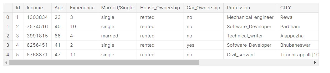
All the dataset columns are not visible here, but I will share the link to the notebook, so please check it from there.
Understanding the Dataset
First, we start with understanding the data set and how is the data distributed.
rows, columns = data.shape
print('Rows:', rows)
print('Columns:', columns)
Output:
- Rows: 252000
- Columns: 13
So, we see that the data is 252000 rows, that is 252000 data points and 13 columns, that is 13 features. Out of13 features, 12 are input features and 1 is output feature.
Now we check the data types and other information.
data.info()
Output:
RangeIndex: 252000 entries, 0 to 251999

Data columns (total 13 columns)
 #   Column             Non-Null Count   Dtype
---  ------             --------------   -----
 0   Id                 252000 non-null  int64
 1   Income             252000 non-null  int64
 2   Age                252000 non-null  int64
 3   Experience         252000 non-null  int64
 4   Married/Single     252000 non-null  object
 5   House_Ownership    252000 non-null  object
 6   Car_Ownership      252000 non-null  object
 7   Profession         252000 non-null  object
 8   CITY               252000 non-null  object
 9   STATE              252000 non-null  object
 10  CURRENT_JOB_YRS    252000 non-null  int64
 11  CURRENT_HOUSE_YRS  252000 non-null  int64
 12  Risk_Flag          252000 non-null  int64
dtypes: int64(7), object(6)
memory usage: 25.0+ MB
So, we see that half the features are numeric and half are string, so they are probably categorical features.
Numerical data is the representation of measurable quantities of a phenomenon. We call numerical data “quantitative data” in data science because it describes the quantity of the object it represents.
Categorical data refers to the properties of a phenomenon that can be named. This involves describing the names or qualities of objects with words. Categorical data is referred to as “qualitative data” in data science since it describes the quality of the entity it represents.
Let us check if there are any missing values in the data.
data.isnull().sum()
Output:
Id                   0
Income               0
Age                  0
Experience           0
Married/Single       0
House_Ownership      0
Car_Ownership        0
Profession           0
CITY                 0
STATE                0
CURRENT_JOB_YRS      0
CURRENT_HOUSE_YRS    0
Risk_Flag            0
dtype: int64
So, there is no missing or empty data here.
Let us check the data column names.
data.columns
Output:
Index(['Id', 'Income', 'Age', 'Experience', 'Married/Single',
       'House_Ownership', 'Car_Ownership', 'Profession', 'CITY', 'STATE',
       'CURRENT_JOB_YRS', 'CURRENT_HOUSE_YRS', 'Risk_Flag'],
      dtype='object')
So, we get the names of the data features.
Analyzing Numerical Columns
First, we start with the analysis of numerical data.
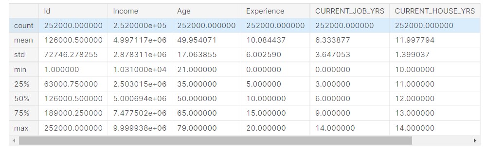
data.describe()
Output:
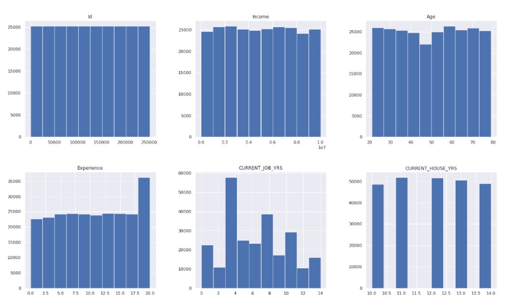
Now, we check the data distribution.
data.hist( figsize = (22, 20) )
plt.show()
Output:
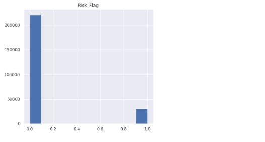
Now, we check the count of the target variable.
data["Risk_Flag"].value_counts()
Output:
0    221004
1     30996
Name: Risk_Flag, dtype: int64
Only a small part of the target variable consists of people who default on loans.
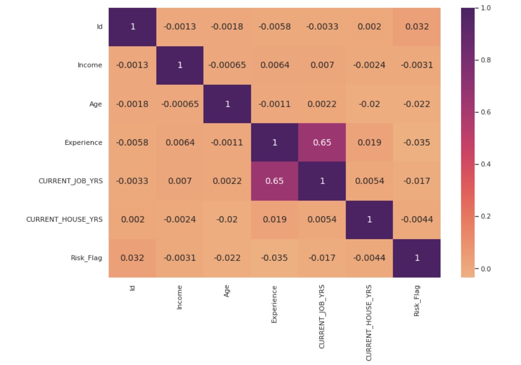
Now, we plot the correlation plot.
fig, ax = plt.subplots( figsize = (12,8) )
corr_matrix = data.corr()
corr_heatmap = sns.heatmap( corr_matrix, cmap = "flare", annot=True, ax=ax, annot_kws={"size": 14})
plt.show()
Output:
Analyzing Categorical Features
Now, we proceed with the analysis of categorical features.
First, we define a function to create the plots.
def categorical_valcount_hist(feature):
    print(data[feature].value_counts())
    fig, ax = plt.subplots( figsize = (6,6) )
    sns.countplot(x=feature, ax=ax, data=data)
    plt.show()
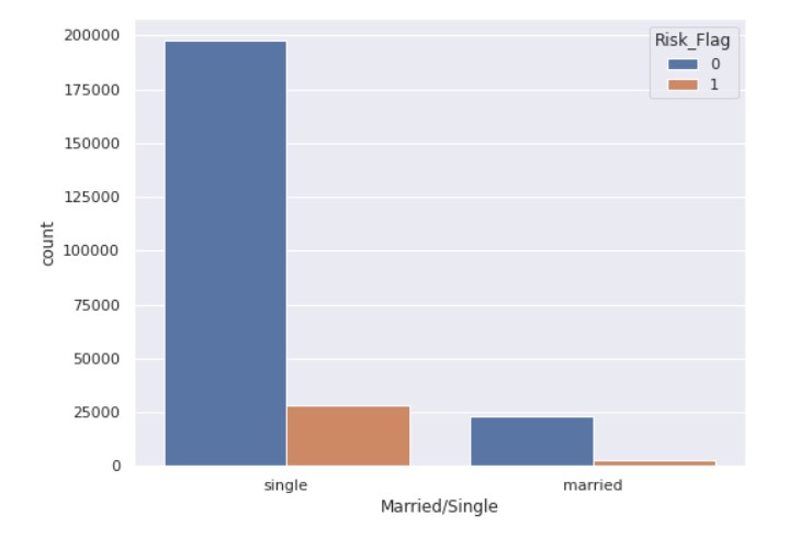
First, we check the count of married people vs single people.
categorical_valcount_hist("Married/Single")
Output:
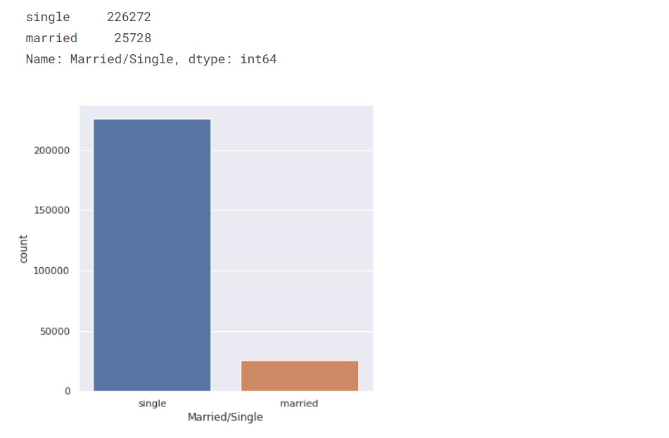
So, the majority of the people are single.
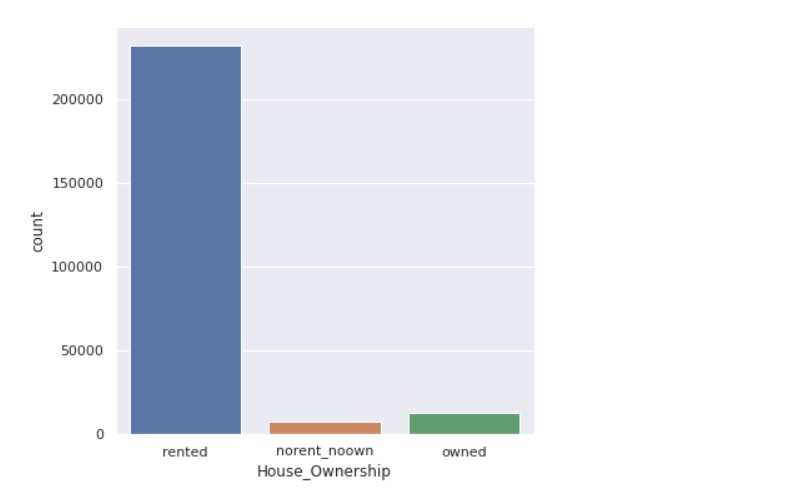
Now, we check the count of house ownership.
categorical_valcount_hist("House_Ownership")
Output:
Now, let us check the count of states.
print( "Total categories in STATE:", len( data["STATE"].unique() ) )
print()
print( data["STATE"].value_counts() )
Output:
Total categories in STATE: 29
Uttar_Pradesh        28400
Maharashtra          25562
Andhra_Pradesh       25297
West_Bengal          23483
Bihar                19780
Tamil_Nadu           16537
Madhya_Pradesh       14122
Karnataka            11855
Gujarat              11408
Rajasthan             9174
Jharkhand             8965
Haryana               7890
Telangana             7524
Assam                 7062
Kerala                5805
Delhi                 5490
Punjab                4720
Odisha                4658
Chhattisgarh          3834
Uttarakhand           1874
Jammu_and_Kashmir     1780
Puducherry            1433
Mizoram                849
Manipur                849
Himachal_Pradesh       833
Tripura                809
Uttar_Pradesh[5]       743
Chandigarh             656
Sikkim                 608
Name: STATE
dtype: int64
Now, we check the count of professions.
print( "Total categories in Profession:", len( data["Profession"].unique() ) )
print()
data["Profession"].value_counts()
Output:
Total categories in Profession: 51
Physician                     5957
Statistician                  5806
Web_designer                  5397
Psychologist                  5390
Computer_hardware_engineer    5372
Drafter                       5359
Magistrate                    5357
Fashion_Designer              5304
Air_traffic_controller        5281
Comedian                      5259
Industrial_Engineer           5250
Mechanical_engineer           5217
Chemical_engineer             5205
Technical_writer              5195
Hotel_Manager                 5178
Financial_Analyst             5167
Graphic_Designer              5166
Flight_attendant              5128
Biomedical_Engineer           5127
Secretary                     5061
Software_Developer            5053
Petroleum_Engineer            5041
Police_officer                5035
Computer_operator             4990
Politician                    4944
Microbiologist                4881
Technician                    4864
Artist                        4861
Lawyer                        4818
Consultant                    4808
Dentist                       4782
Scientist                     4781
Surgeon                       4772
Aviator                       4758
Technology_specialist         4737
Design_Engineer               4729
Surveyor                      4714
Geologist                     4672
Analyst                       4668
Army_officer                  4661
Architect                     4657
Chef                          4635
Librarian                     4628
Civil_engineer                4616
Designer                      4598
Economist                     4573
Firefighter                   4507
Chartered_Accountant          4493
Civil_servant                 4413
Official                      4087
Engineer                      4048
Name: Profession
dtype: int64
Data Analysis
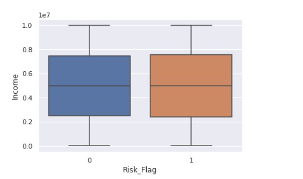
Now, we start with understanding the relationship between the different data features.
sns.boxplot(x ="Risk_Flag",y="Income" ,data = data)
Output:
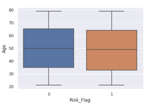
Now, we see the relationship between the flag variable and age.
sns.boxplot(x ="Risk_Flag",y="Age" ,data = data)
Output:
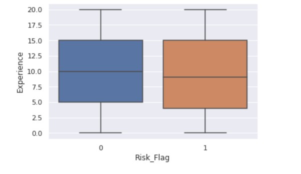
sns.boxplot(x ="Risk_Flag",y="Experience" ,data = data)
Output:
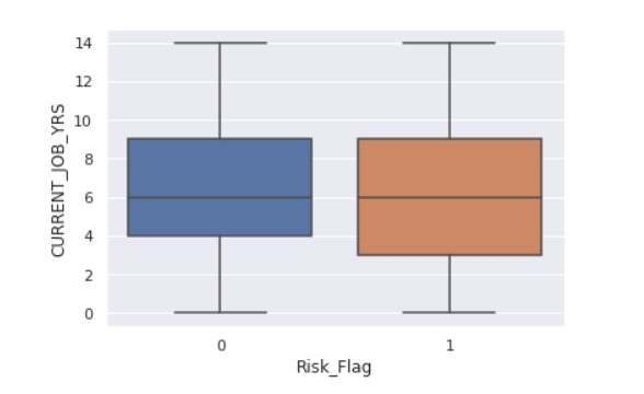
sns.boxplot(x ="Risk_Flag",y="CURRENT_JOB_YRS" ,data = data)
Output:
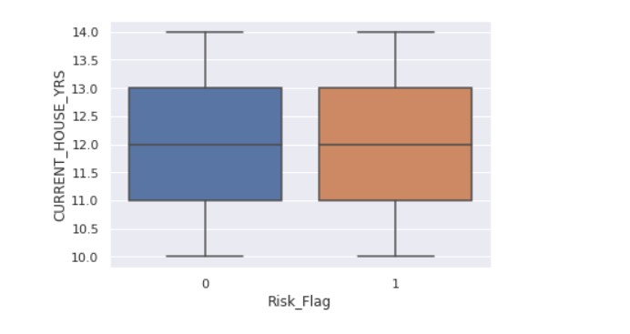
sns.boxplot(x ="Risk_Flag",y="CURRENT_HOUSE_YRS" ,data = data)
Output:
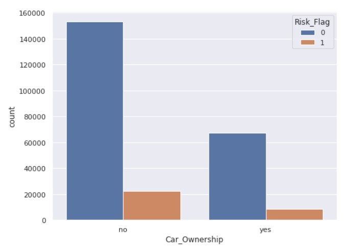
fig, ax = plt.subplots( figsize = (8,6) )
sns.countplot(x='Car_Ownership', hue='Risk_Flag', ax=ax, data=data)
Output:
fig, ax = plt.subplots( figsize = (8,6) )
sns.countplot( x='Married/Single', hue='Risk_Flag', data=data )
Output:
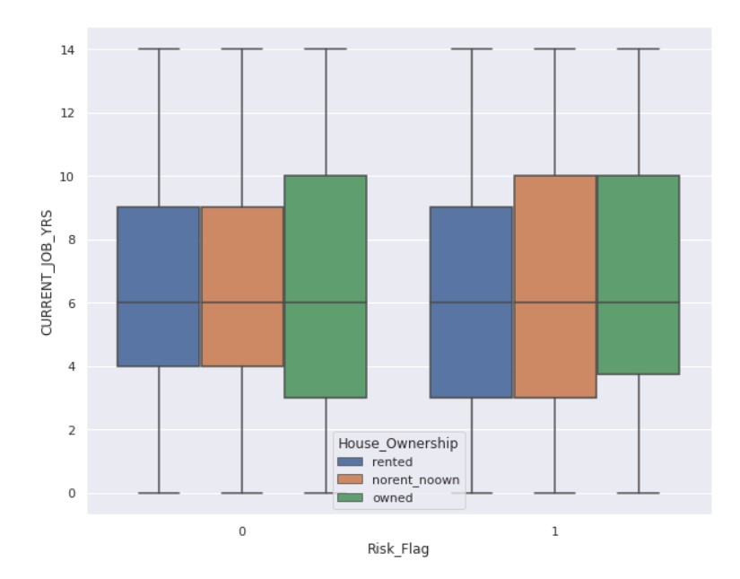
fig, ax = plt.subplots( figsize = (10,8) )
sns.boxplot(x = "Risk_Flag", y = "CURRENT_JOB_YRS", hue='House_Ownership', data = data)
Output:
Encoding
Data preparation is a required process in the field of data science before moving on to modelling. In the data preparation process, we must complete a number of tasks. One of these critical responsibilities is the encoding of categorical data. We all know that most data in real life contains categorical string values, and most machine learning models handle only integer values or other understandable formats. In essence, all models execute mathematical operations that various tools and methodologies can perform.
Encoding categorical data is the process of turning categorical data into integer format so that data with transformed categorical values may be fed into models to increase prediction accuracy.
We will apply encoding to the categorical features.
from sklearn.preprocessing import LabelEncoder
from sklearn.preprocessing import OneHotEncoder
import category_encoders as ce
label_encoder = LabelEncoder() for col in ['Married/Single','Car_Ownership']: data[col] = label_encoder.fit_transform( data[col] )
onehot_encoder = OneHotEncoder(sparse = False)
data['House_Ownership'] = onehot_encoder.fit_transform(data['House_Ownership'].values.reshape(-1, 1) )
high_card_features = ['Profession', 'CITY', 'STATE']
count_encoder = ce.CountEncoder()
# Transform the features, rename the columns with the _count suffix, and join to dataframe
count_encoded = count_encoder.fit_transform( data[high_card_features] )
data = data.join(count_encoded.add_suffix("_count"))
data= data.drop(labels=['Profession', 'CITY', 'STATE'], axis=1)
After the feature engineering part is complete, we shall split the data into training and testing sets.
Splitting the Data into Train and Test Splits
The train-test split is used to measure the performance of machine learning models relevant to prediction-based Algorithms/Applications. This approach is a quick and simple procedure that allows us to compare our own machine learning model outcomes to machine results. By default, the Test set is made up of 30% of the real data, whereas the Training set is made up of 70% of the actual data.
To assess how effectively our machine learning model works, we must divide a dataset into training and testing sets. The train set is used to train the Machine Learning model, and its statistics are known. The second set is known as the test data set, and it is only utilized for predictions.
It is an important part of the ML chain.
x = data.drop("Risk_Flag", axis=1)
y = data["Risk_Flag"]
from sklearn.model_selection import train_test_split
x_train, x_test, y_train, y_test = train_test_split(x, y, test_size = 0.2, stratify = y, random_state = 7)
We have taken the test size to be 20% of the entire data.
Random Forest Classifier
Tree-based algorithms, such as random forests, play a crucial role in loan default prediction and credit risk assessment. These algorithms are adept at handling both classification and regression tasks, making them valuable in analyzing loan applications. By generating predictions based on training samples, they offer high accuracy and stability, crucial for identifying potential defaulters.
In the context of loan default prediction, tree-based algorithms help minimize false negatives and false positives, ensuring robust risk assessment. While individual decision trees may overfit training data, random forests mitigate this issue by averaging predictions from multiple trees, resulting in improved prediction accuracy.
In academic research, studies exploring the efficacy of tree-based algorithms in loan default prediction can be found in reputable journals. Authors often provide DOIs for their work, facilitating citation and further research in this area. Additionally, comparisons between tree-based models and logistic regression models may offer insights into the strengths and limitations of each approach in credit risk assessment.
Now, we train the model and perform the predictions.
from sklearn.ensemble import RandomForestClassifier
from imblearn.over_sampling import SMOTE
from imblearn.pipeline import Pipeline
rf_clf = RandomForestClassifier(criterion='gini', bootstrap=True, random_state=100)
smote_sampler = SMOTE(random_state=9)
pipeline = Pipeline(steps = [['smote', smote_sampler],
                             ['classifier', rf_clf]])
pipeline.fit(x_train, y_train)
y_pred = pipeline.predict(x_test)
Now, we check the accuracy scores.
from sklearn.metrics import confusion_matrix, precision_score, recall_score, f1_score, accuracy_score, roc_auc_score
print("-------------------------TEST SCORES-----------------------")
print(f"Recall: { round(recall_score(y_test, y_pred)*100, 4) }")
print(f"Precision: { round(precision_score(y_test, y_pred)*100, 4) }")
print(f"F1-Score: { round(f1_score(y_test, y_pred)*100, 4) }")
print(f"Accuracy score: { round(accuracy_score(y_test, y_pred)*100, 4) }")
print(f"AUC Score: { round(roc_auc_score(y_test, y_pred)*100, 4) }")
Output:
-------------------------TEST SCORES-----------------------
Recall: 54.1378
Precision: 54.3306
F1-Score: 54.234
Accuracy score: 88.7619
AUC Score: 73.8778
The accuracy scores might not be up to the mark, but this is the overall process of predicting loan default.
Code: Here
Conclusion
In summary predicting loan default involves thorough exploratory data analysis (EDA) to understand dataset characteristics. Utilizing Python libraries and techniques like boosting, random forest classifiers, and logistic regression, classification models are developed, leveraging artificial intelligence algorithms. Evaluation metrics such as accuracy, precision, recall, F1-score, and AUC assess model performance in binary classification tasks. International conferences on data science and AI foster collaboration and innovation in risk assessment and management. This integrated approach enables effective prediction of loan default, crucial for financial sector risk management.
Key Take Away
- The Random Forest approach is appropriate for classification and regression tasks on datasets with many entries and features that are likely to have missing values when we need a highly accurate result while avoiding overfitting.
- Furthermore, the random forest provides relative feature significance, enabling you to select the most important features. It is more interpretable than neural network models but less interpretable than decision trees.
- In the case of categorical features, we need to perform encoding so that the ML algorithm can process them.
- Predicting Loan Default is highly dependent on the demographics of the people, people with lower income are more likely to default on loans.
We are able to successfully perform the classification task using Random Forest Classifier. Hope you liked my article on predicting loan default.
Frequently Asked Questions
A. Loan default prediction is crucial for financial institutions to assess the risk associated with lending money to individuals or businesses. By accurately predicting the likelihood of default, lenders can make informed decisions regarding loan approval, interest rates, and loan terms, ultimately minimizing potential losses and maintaining a healthy loan portfolio.
A. There isn’t a universally “best” model for predicting loan defaults as it depends on various factors such as the nature of the dataset, the available features, and the specific requirements of the lender. However, commonly used models for loan default prediction include logistic regression, decision trees, random forests, gradient boosting machines, and neural networks.
A. Probability of default prediction refers to estimating the likelihood or probability that a borrower will fail to meet their loan obligations. This prediction is typically expressed as a numerical value ranging from 0 to 1, where 0 indicates low risk (unlikely to default) and 1 indicates high risk (likely to default). It serves as a quantitative measure for assessing credit risk and informing lending decisions.
The loan default prediction dataset typically consists of historical loan data including various borrower attributes such as credit score, income, employment status, debt-to-income ratio, loan amount, loan term, and repayment history.
The media shown in this article is not owned by Analytics Vidhya and are used at the Author’s discretion.
Prateek is a final year engineering student from Institute of Engineering and Management, Kolkata. He likes to code, study about analytics and Data Science and watch Science Fiction movies. His favourite Sci-Fi franchise is Star Wars. He is also an active Kaggler and part of many student communities in College.


