Gaussian Naive Bayes Algorithm for Credit Risk Modelling

This article was published as a part of the Data Science Blogathon.

Overview

 

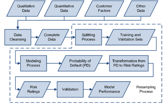
In recent years, corporate banks’ credit evaluations have become more sophisticated. Credit evaluations have progressed from being subjective decisions by the bank’s credit experts to a more statistically advanced evaluation. Banks rapidly recognize the increased need for comprehensive credit risk modelling. Now we can build a model for credit risk by using naive Bayes.

The Naive Bayes algorithm is a straightforward and quick machine learning algorithm that is frequently used for real-time predictions. It’s enjoyable to learn because of its strong ties to probability principles, and it’ll aid you in making informed judgments throughout your data science journey.  Are you ready to build a model for credit risk by using naive Bayes? Come on, Let’s turn to implement the model.

Naive Bayes Algorithm

Naïve Bayes is a probabilistic algorithm that is based on the concept of conditional probability. We know it not only for its simplicity but also for its speed.

We also defined it as an algorithm is a simple and fast machine learning algorithm that is often favored in cases of real-time predictions.

What is probability?

It refers to the possibilities or likelihood of an event occurring as a probability.

P(A/B) is the conditional probability of A given B, or the likelihood of event A if event B has already occurred. Because we already know that B has happened when we experiment, the number of alternative outcomes for the event has been limited. As a result, given that B has already occurred, the unconditional probability has now changed to a conditional probability.

We define the conditional probability as:

𝑃(𝐴/𝐵) = 𝑃(𝐴 ∩ 𝐵) 𝑃(𝐵)

Where 𝑃(𝐴 ∩ 𝐵) represents the joint probability, i.e. probability, of both events happening together.

Types of Naïve Bayes

There are three main types of Naïve Bayes which are listed below:

1. Gaussian Naïve Bayes

2. Multinomial Naïve Bayes

3. Bernoulli Naïve Bayes

Gaussian Naïve Bayes algorithm

In Gaussian Naïve Bayes, the assumption is made that the continuous numerical attributes are distributed normally. The attribute is first segmented based on the output class, and then the variance and mean of the attribute are calculated for each class.

Multinomial Naïve Bayes algorithm

We prefer the multinomial Naïve Bayes model when the data is multinomially distributed. The feature vectors represent the frequency with which a multinomial has generated a certain event. We mostly used the multinomial Naïve Bayes algorithm in cases of text classification.

Bernoulli Naïve Bayes’ algorithm

In Bernoulli Naïve Bayes algorithm, the features are distributed according to multivariate Bernoulli distributions. This means that there may be multiple features, but each one will be an independent Boolean variable. Hence, it requires the samples to be binary-values. Similar to the multinomial algorithm, the Bernoulli algorithm is popular for text classification, where binary occurrences are used in place of term frequencies.

Naïve Bayes Classifier

It is a supervised machine learning algorithm for classification based on Bayes’ theorem. The algorithm learns the probability of data instances belonging to a particular class. Hence, it is a probabilistic classifier.

The reason for calling it “naïve” is that it assumes that the occurrence of a particular feature (X) is independent of the occurrence of any other features (any other Xs). For example, we can predict fruit as an apple if it is red, round, and 2 inches in width. These features independently contribute to the probability that the predicted fruit is an apple, even though these features depend on each other.

This can also be considered as an advantage since the Naïve Bayes algorithm requires only a small amount of training data for the estimation of the parameters of the algorithm.

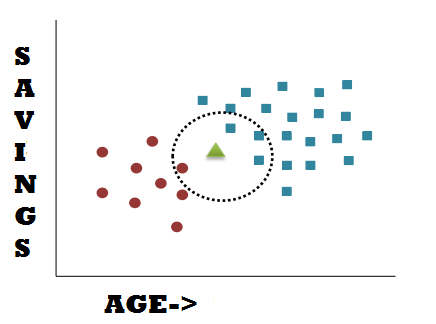
In the above picture, the red circle category represents the person who does not own a bike, whereas the blue square category represents the person who owns a bike. There is another data point marked by the Green triangle. How do we find out in which category does the data point lie or if the person owns a bike?

Let us use the Naïve Bayes algorithm to solve this problem. First, we calculate the probability of a person owning a bike or not. The total data points are 30, red points are 9 and blue points are 21.

𝑃(𝑁𝑜 𝑏𝑖k𝑒) = 9/30 𝑃(𝑏𝑖k𝑒) = 21/30

The new data point is like the data points in that circle, it may have any radius value. The marginal probability says that if we add a new point,

𝑃(𝑃𝑜𝑖𝑛𝑡) = 𝑁𝑢𝑚𝑏𝑒𝑟 𝑜𝑓 𝑂𝑏𝑠𝑒𝑟𝑣𝑎𝑡𝑖𝑜𝑛𝑠 𝑖𝑛 𝑐𝑖𝑟𝑐𝑙𝑒/ 𝑇𝑜𝑡𝑎𝑙 𝑂𝑏𝑠𝑒𝑟𝑣𝑎𝑡𝑖𝑜𝑛𝑠 = 4/30

The next probability that we will calculate will say that the new data point will lie in the circle given that the person does not own a bike.

𝑃 ( 𝑃𝑜𝑖𝑛𝑡 / 𝑁𝑜 𝑏𝑖k𝑒 ) = 𝑁𝑢𝑚𝑏𝑒𝑟 𝑜𝑓 𝑁𝑜 𝑏𝑖k𝑒 𝑂𝑏𝑠𝑒𝑟𝑣𝑎𝑡𝑖𝑜𝑛𝑠 𝑖𝑛 𝑐𝑖𝑟𝑐𝑙𝑒 /𝑇𝑜𝑡𝑎𝑙 𝑂𝑏𝑠𝑒𝑟𝑣𝑎𝑡𝑖𝑜𝑛𝑠 𝑜𝑓 𝑁𝑜 𝑏𝑖k𝑒 = 1/9

The posterior probability is given by,

𝑃(𝑁𝑜 𝑏𝑖k𝑒/𝑃𝑜𝑖𝑛𝑡) = 1 / 4 = 0.25

So there is a 25% chance that the given data point/person does not own a bike. Calculate the other posterior probability.

𝑃(𝑏𝑖k𝑒/𝑃𝑜𝑖𝑛𝑡) = 3 / 4 = 0.75

And there’s a 75% probability the person owns a bike. As a result, the new person is more likely to own a bike. After then, we will classify the point as a person who owns a bike. The Naive Bayes algorithm works in this way.

Importing packages:

Import the packages
import numpy as np 
import pandas as pd 
from scipy.stats import randint
import pandas as pd 
import matplotlib.pyplot as plt 
from pandas import set_option
plt.style.use('ggplot')

from sklearn.model_selection import train_test_split 
from sklearn.linear_model import LogisticRegression 
from sklearn.feature_selection import RFE
from sklearn.model_selection import KFold 
from sklearn.model_selection import GridSearchCV 
from sklearn.model_selection import RandomizedSearchCV  
from sklearn.preprocessing import StandardScaler 
from sklearn.pipeline import Pipeline 
from sklearn.ensemble import RandomForestClassifier
import xgboost as xgb
from xgboost import XGBClassifier

from sklearn.model_selection import cross_val_score
from sklearn.metrics import confusion_matrix
from sklearn.neighbors import KNeighborsClassifier 
from sklearn.tree import DecisionTreeClassifier
from sklearn.ensemble import ExtraTreesClassifier
from sklearn.feature_selection import SelectFromModel
from sklearn import metrics 
import warnings
warnings.filterwarnings("ignore", category=FutureWarning)

from sklearn.metrics import classification_report

Data Preprocessing

Download the dataset:

The first step towards solving any problem with machine learning is to understand and prepare the data.

The dataset is available in kaggle, and we can download it from the link

https://www.kaggle.com/uciml/default-of-credit-card-clients-dataset/version/1?select=UCI_Credit_Card.csv

After downloading the dataset, we can import the dataset by using the pandas’ framework. The dataframe is loaded in the BankCredit variable.

BankCredit = pd.read_csv("UCI_Credit_Card.csv")

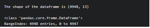
Use the shape attribute of Pandas Dataframe to check the shape of the dataframe.

To print the shape of the dataframe

print(f'The shape of the dataframe is {BankCredit.shape}')
print()

Output

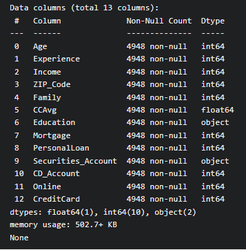
Use info() function of Pandas Dataframe to display data types of each column.

print(BankCredit.info())
print()

Output

Use replace function from Python to replace the ? with Numpy NaN. Remember to use the inplace attribute to replace the original dataframe.

BankCredit.replace(to_replace='?', value=np.NaN, inplace=True)

Output

We can see the output columns with ‘?’ is replaced by ‘NaN’

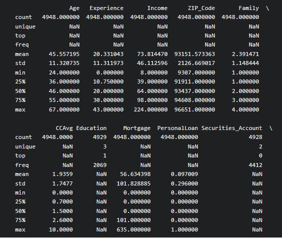
Use describe a method to get a descriptive summary of the features of the dataset.

print(BankCredit.describe(include='all'))
print()

Exploratory Data analysis

The next step is to perform Exploratory Data Analysis. Here, Count plots will display categorical target variables. Histograms are used to display the distribution of the other variables.

The first step is to check the count of categories in the target variable.

Use value_counts() method to count the number of categories in the target variable

The below code will print the number of values in each category of the target variable (Income)

Also, It is important to check the null values in the dataset, so we use the isnull method to check for missing values

print(BankCredit['CreditCard'].value_counts())

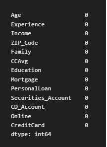
print(BankCredit.isnull().sum()

output

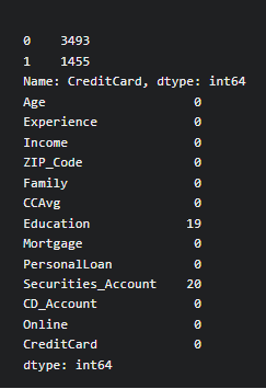
We have missing values in columns ‘Education’ and ‘Securitiess_Account’.

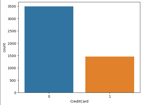
Next, to visualize the output using a bar chart, we use the count plot method of the seaborn library to display the Bar chart of the target variable

sns.countplot(x='CreditCard', data=BankCredit, linewidth=3)
plt.show()

Output

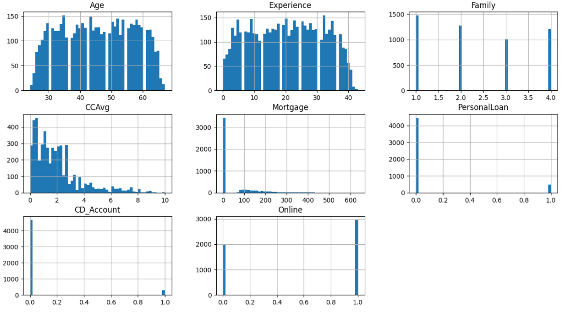
To display the histogram of the variables of the dataset, we use the hist method to display the histogram of the features selected for the dataframe.

BankCredit[['Age', 'Experience', 'Family', 'CCAvg', 'Mortgage','PersonalLoan', 'CD_Account', 'Online']].hist(bins=50, figsize=(15,8))
plt.show()

Model Train and test split

1) First, we should replace the missing values with the most frequently occurring category

2) We have to specify which one is dependent and independent variables then we have to split the dataset into train and test

3) To treat categorical variables for missing data with the mode of the columns

After analyzing the missing data in the dataset, columns ‘Education’ and ‘Securities_Account’ have the missing values, so we can use mode() statistics to replace the missing values in categorical variables.

BankCredit['Education'].fillna(BankCredit['Education'].mode()[0], inplace=True)
BankCredit['Securities_Account'].fillna(BankCredit['Securities_Account'].mode()[0], inplace=True)

To recheck whether we correctly replaced missing values, we use the isnull() function again to check for missing values

print(BankCredit.isnull().sum())

Output

After treating the missing data using mode method, the missing data are replaced with the mode. If we check for missing value, it shows null missing value.

To declare the independent (X) and the dependent (y) variable, we use the drop() method to remove [‘Experience’,’ZIP_Code’,’CreditCard’] features and use the rest of the features as independent features. Use [‘CreditCard’] as the dependent variable.

X = BankCredit.drop(['Experience','ZIP_Code','CreditCard'], axis=1)
y = BankCredit['CreditCard']

To Split the data, we use the train_test_split class from sklearn.model_selection module to split the dataset into the train and test.

from sklearn.model_selection import train_test_split
X_train, X_test, y_train, y_test = train_test_split(X, y, test_size=0.3, random_state=42, stratify=y)

To Fit the Naive Bayes Model

The representation of categorical data can be more expressive with one-hot encoding. Many machine learning algorithms cannot operate directly with categorical data. The categories must be numerically transformed.

To Perform One-Hot Encoding, we use one hot encoder class from sklearn.preprocessing module to perform one Hot Encoding of the categorical variables. With One hot encoding, we get one column per category for a variable.

from sklearn.preprocessing import OneHotEncoder
cols = ['Family','Education','PersonalLoan','Securities_Account','CD_Account','Online']
encoder = OneHotEncoder(sparse=False)
X_train = encoder.fit_transform(X_train[cols])
X_test = encoder.transform(X_test[cols])

To scale the input features using MinMaxScaler, we Use MinMaxScaler to transform the independent features of training and testing data.

from sklearn.preprocessing import MinMaxScaler
scaler =  MinMaxScaler()
X_train = scaler.fit_transform(X_train)
X_test = scaler.transform(X_test)

After performing the above steps, we have to create an instance of the Naive Bayes algorithm. To create it, we use the GaussianNB class from sklearn.naive_bayes package to create an instance of the algorithm.

from sklearn.naive_bayes import GaussianNB

model_gnb = GaussianNB()

Our next step is to fit the algorithm on the training dataset. To perform this, we use the fit method to fit the algorithm on the training data.

model_gnb.fit(X_train, y_train)

Efficiency of the Naive Bayes Model

After fitting the model on the training data, the next step is to make predictions and test the performance of the model that has been built.

Finally, to make predictions on the training data. We use predict method to make predictions on the test data. After that, we have to calculate the accuracy of the model. We use accuracy_score class from sklearn.metrics to measure the accuracy.

y_pred = model_gnb.predict(X_test)
#To measure Accuracy
from sklearn.metrics import accuracy_score
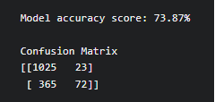
print(f'Model accuracy score: {100*accuracy_score(y_test, y_pred):0.2f}%')
print()

Finally, we use confusion_matrix class from sklearn.metrics to calculate the confusion matrix for the model.

from sklearn.metrics import confusion_matrix
cm = confusion_matrix(y_test, y_pred)
print('Confusion Matrix')
print(cm)

Output

 

Inference of the Naive Bayes model

This model gives 73.8% accuracy and we can improve the accuracy by using hyperparameter optimization method.

1) The probability of the hypothesis multiplies the prior probability of a hypothesis, given the training data.

2) The output is not only classification but also a probability distribution representing all classes as well.

3) With each data instance, the prior and the likelihood can be updated incrementally.

Conclusion

Naïve Bayes is fast in predicting the class of the dataset. Hence, it can be used in real-time for making predictions. Finally, we have trained and built a model for credit card modeling using Naive Bayes.

I hope this article will be more illustrative and stimulating!

If you have further queries, please post them in the comments section. If you are interested in reading my other articles, check them out here!

Thank you for reading.

About Myself

My name is Lavanya, and I’m from Chennai, India. I used to surf through many new technology concepts as a passionate writer and enthusiastic content creator. I’m pursuing a B.E., In Computer Science Engineering and have a strong interest in data engineering, machine learning, data science, artificial intelligence, and Natural Language Processing,

LinkedIn URL: https://www.linkedin.com/in/lavanya-srinivas-949b5a16a/

Email: [email protected]

The media shown in this article is not owned by Analytics Vidhya and are used at the Author’s discretion.