Cryptocurrency Investing Python Strategy
This article was published as a part of the Data Science Blogathon.
Introduction
Investing Strategies are essential since they determine whether you gain or lose money. Investing strategies vary depending on the investor’s risk appetite and goals (long term or short term). Cryptocurrencies are a type of digital currency that may be utilized as payment methods without the intervention of a third party. Cryptocurrencies as an asset class that have returned over 10,000% to investors in a single year.
The Fear and Greed Index is a sort of indicator that monitors market sentiment. Social media, Google Trends, market volatility, market volume, dominance, and surveys all contribute to the Fear and Greed Index’s value. Fear and Greed values indicate if the market is in Extreme Fear, Fear, Neutral, Greed, and Extreme Greed. “Extreme Fear” suggests that the emotion is too fearful, indicating a potential buying opportunity, whereas “Extreme Greed” implies that the market is about to correct. To know more about the Fear and Greed Indication, please feel free to check out Alternative.me.
In this project, we will examine the advantages of employing a well-known investment method known as Dollar Cost Averaging (DCA) with the use of the Fear and Greed Index. This investing strategy can be used with other investing strategies to achieve even greater results. The analysis highlights Bitcoin’s long-term performance and demonstrates the long-term potential of DCA during “Extreme Fear” times.
Libraries Used
The libraries used in this project make data analysis extremely simple. These libraries may be obtained by executing the pip command in the terminal:
pip install library_name
The libraries that are used are briefly described below:
| Library | Description |
| Pandas | To manipulate and analyze DataFrames |
| json | To store and transfer the data into your Python project |
Dataset and Data Description
For this project, we require two sets of data:
- Fear and Greed Data
- Bitcoin Price History Data
Fear and Greed Index Data
The Fear and Greed data used in the project has been taken from Alternative.me Fear and Greed Index API. You can view the data used in the project by clicking on this link. Then hold the ‘Ctrl’ and ‘S’ buttons simultaneously to save and download the data in the desired folder.
The data in this dataset consists of ‘value’, ‘value classification’, and ‘timestamp’. We will be using value classification and timestamp for this project.
Feel free to check out the Alternative.me a website for other Fear and Greed Index API data.
Bitcoin Price History Data
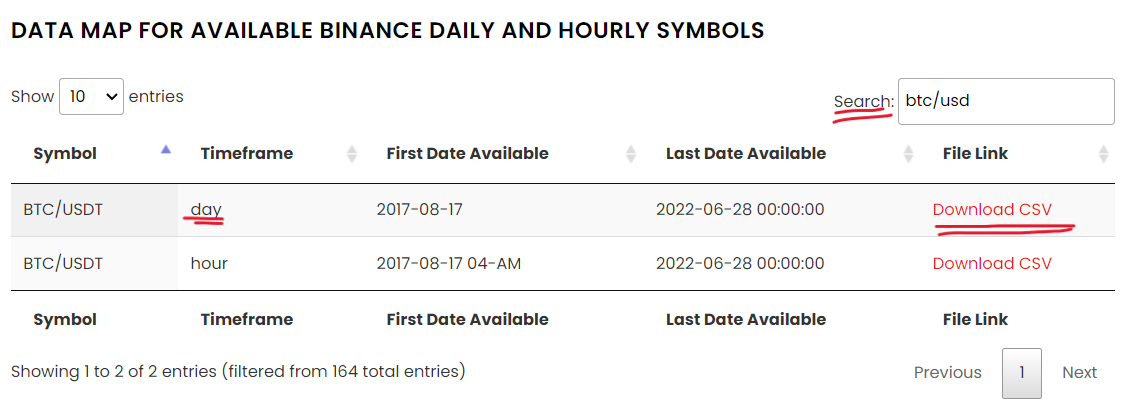
Bitcoin’s Price History data can be downloaded from the cryptodatadownload website.
The data we have used in this project is data of Bitcoin from the Binance exchange. To head to the download site click here. On reaching this page, in the search bar, search for ‘btc/usdt’ and click on the download button for the timeframe showing ‘daily’. Or click here.
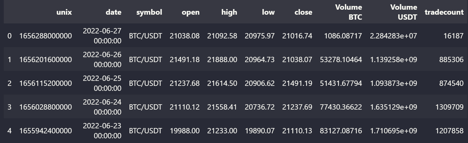
The data in this dataset consists of ‘unix’, ‘date’, ‘symbol’, ‘open’, ‘high’, ‘low’, ‘close’, ‘Volume BTC’, ‘Volume USDT’ and ‘tradecount’. We will be using ‘date’ and ‘open’ in this project.
Feel free to check out the cryptodatadownload website to download crypto data to use it for your project from a number of exchanges (Kraken, Gemini, Coinbase, and more) and a number of different crypto coins and tokens (Ethereum, Dogecoin, Solana).
Importing Packages
Importing Dataset
btc=pd.read_csv("Binance_BTCUSDT_d.csv")


#need to load the json file first

fear = json.load(open('Fear_Data.json'))


#convert our data in json to dataframe

df = pd.DataFrame(fear["data"])
Viewing Data
btc.head()
df.head()
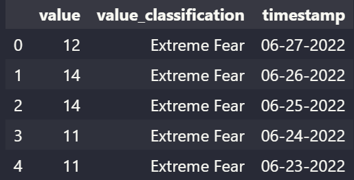
From the above tables, we can view the first 5 rows of the Bitcoin Price Dataset and the Fear and Greed Index datasets and get a brief overview of the data present.
Viewing Datatypes of all columns
btc.info()
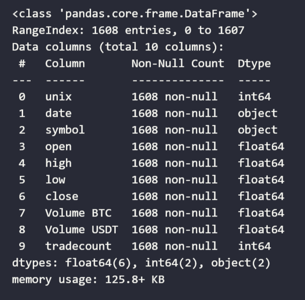
Here, we can notice the datatype of “date” is ‘object’ in the Bitcoin Price dataset, hence we need to convert it into the ‘date’ datatype (Which we will do in the “Working on Data” section).
You will see a similar result for the datatypes for Fear and Greed Index datasets for the ‘timestamp’ column after executing the df.info() function.
Working on Data
Converting ‘date’ and ‘timestamp’ column dtype from object to date
btc["date"]=pd.to_datetime(btc["date"])
df["date"]=pd.to_datetime(df["timestamp"])
Once this code is executed, if you try executing the .info() function on any of the datasets, you will notice the datatype of the ‘date’ and ‘timestamp’ column changed from ‘object’ to ‘datetime64[ns]’ for both the datasets.
Finding number of times the market was in “Extreme Fear”
'''c=0

for i in range(len(fear)):

if fear.loc[i,'value_classification']=='Extreme Fear':

c+=1

print(c)'''
fear['value_classification'].value_counts()['Extreme Fear']
We get output as 432 indicating there have been 432 times the market was in “Extreme Fear” from 01/02/2018 to 27/06/2022.
Storing the dates into a list when there was “Extreme Fear” in the market
extreme_fear_date=[]
for i in range(len(df)):
    if df.loc[i,'value_classification']=='Extreme Fear':
        extreme_fear_date.append(df.loc[i,'date'])
After executing this code, the ‘extreme_fear_date’ will consist of all the dates when the market was in “Extreme Fear”.
Checking if the size of the ‘extreme_fear_date’ is equal to the number of times the market was in “Extreme Fear”
len(extreme_fear_date)
The result for this code will also be 432, confirming that our code is accurate.
Reversing the contents of extreme_fear_date
We are reversing the extreme_fear_date list since we want the date starting from 2018-02-02 and not 2022-06-27.
ext=extreme_fear_date[::-1]
Investment Results
Current Portfolio Value
In this section, we will see the power of buying BTC worth $10 for each day at the opening price (i.e at 12am) when the market was in “Extreme Fear”.
j=431

qty=0

#iterating through the dattaset backwards so to get 2018 data first

for i in range(len(btc)-1,-1,-1):

if j>=0:

if(btc.loc[i,'date']==extreme_fear_date[j]):

price=btc.loc[i,'open']

qty=qty+(10/price)

j-=1


#calculating investment results

qty=round(qty,2)

profit=round(qty*21000-10*432,2)

capital=10*432

current_value=round(qty*21000-10*432,2)+10*432

roi=round((profit/capital)*100,2)


#printing investment results

print("Quantity of BTC -",qty)

print("Initial Investment - $",capital)

print("Unrealised Profit - $",profit)

print("Current Value - $", current_value)

print("Return on Intrest (ROI) -",roi,"%")
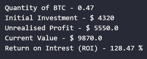
From the above code, we can see that we are sitting at an unrealized profit of $5550.0 which gives us a Return on Investment (ROI) of 128.47%.
Portfolio Value if sold at Top
#max value of portfolio

max_portfolio=max(newdf['Current Value'])

days_invested=1


#need to find quantity of BTC owned at time of selling at top

for i in range(len(newdf)):

if newdf.loc[i,'Current Value']==max_portfolio:

qty=newdf.loc[i,'Quantity']

days_invested=i

break


#calculating investment results

capital=10*days_invested

profit=round(max_portfolio*qty-capital,2)

portfolio_value=round(max_portfolio*qty,2)

roi=round((profit/capital)*100,2)


#printing investment results

print("Quantity of BTC -",round(qty,2))

print("Initial Investment - $",capital)

print("Portfolio Value - $",portfolio_value)

print("Realised Profit - $",profit)

print("Return on Intrest (ROI) -",roi,"%")
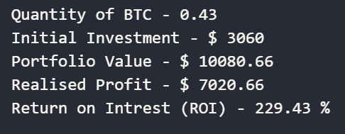
From the above code, we can see that if we sold at the top we would be sitting at a profit of $7020 getting a Return on Investment (ROI) of 229.43%.
Investment Results (Graphically)
In this section, we will plot our portfolio value over time from 2018-02-02 to 2022-06-27. We have created new lists consisting of the required values and inserted them into a new data frame.
j=431

qty=0

count=0

quant=[] #quantity of BTC owned over time

invested=[] #total amount invested over time

btc_price=[] #BTC price when we bought it


for i in range(len(btc)-1,-1,-1):

if j>=0:

if(btc.loc[i,'date']==extreme_fear_date[j]):

price=btc.loc[i,'open']

btc_price.append(price)

qty=qty+(10/price)

quant.append(qty)

j-=1

count+=1

invested.append(count*10)
Creating the Data Frame
newdf=pd.DataFrame(list(zip(ext, quant,invested,btc_price)),columns =['Date', 'Total Quantity','Total Invested','Price'])

newdf["Current Value"]=newdf['Price']*newdf['Quantity']

newdf
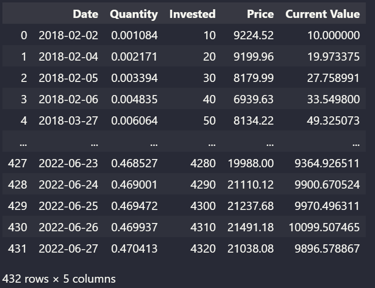
After executing this code, you have created a new Data Frame consisting of ‘Date’, ‘Quantity’, ‘Invested’ and ‘Price.
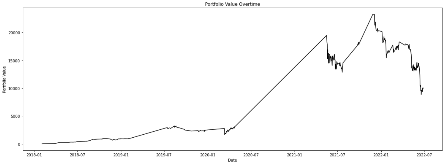
Plotting Portfolio Value Overtime
plt.figure(figsize=(20,7))

plt.plot(newdf['Date'],newdf['Current Value'],color="black")

plt.xlabel("Date")

plt.ylabel("Portfolio Value")

plt.title("Portfolio Value Overtime")
Conclusion
To summarize, using the Fear and Greed Index, an investor has the ability to achieve good long-term returns. However, this is NOT financial advice, all the work done here is for purely educational purposes. An investor should conduct thorough research before investing in any project. This is only one of several investment strategies that an investor may combine with others to achieve even greater results. This analysis highlights Bitcoin’s long-term performance and demonstrates the long-term potential of DCA during “Extreme Fear” times.
Key Takeaways:
- Investing strategies determine whether you gain or lose money.
- The Fear and Greed Index is a sort of indicator that monitors market sentiment.
- We convert the “date” data type from an object into a date datatype to make working on data more simple.
- We have used multiple lists to store various kinds of information on the datasets.
- If we use the Fear and Greed metric and buy BTC worth 10$ daily whenever the Fear and Greed Index says “Extreme Fear”, we will be sitting at an ROI of approximately 128%.
- If we use the Fear and Greed metric and buy BTC worth 10$ daily whenever the Fear and Greed Index says “Extreme Fear” and sold our investment at the extreme top, we would have got an ROI of approximately 229%.
- When the market is down, DCA is an excellent Investing strategy.
- THIS IS NOT A FINANCIAL ADVICE.
The media shown in this article is not owned by Analytics Vidhya and is used at the Author’s discretion.


