This article was published as a part of the Data Science Blogathon
Introduction
Google’s BigQuery is an enterprise-grade cloud-native data warehouse. BigQuery was first launched as a service in 2010, with general availability in November 2011. Since its inception, BigQuery has evolved into a more economical and fully managed data warehouse that can run lightning-fast interactive and ad-hoc queries on petabyte-sized datasets. BigQuery also integrates with various Google Cloud Platform (GCP) services and third-party tools, making it more useful.
rverless, more precisely, data warehouse as a service. There are no servers to manage or database software to install. Instead, BigQuery works on the underlying software and infrastructure, including and high availability. The pricing model is pretty simple – you pay $5 for every 1 TB of data processed. In addition, BigQuery offers a simple client interface that allows users to run interactive queries.
Overall, you don’t need to know much about the underlying architecture of BigQuery or how the service works under the hood. That’s the whole idea of BigQuery – you don’t have to worry about architecture and operation. However, to get started with BigQuery, you need to be able to import data into BigQuery and then be able to write queries using the SQL dialects that BigQuery offers.
A good understanding of BigQuery architecture helps implement various BigQuery best practices, including cost management, query performance optimization, and storage optimization. Understanding how BigQuery allocates resources and the relationship between the number of blocks and query performance is beneficial for the best query performance.
Architecture at a high level
BigQuery is built on Dremel technology, produced in-house at Google since 2006. Dremel is Google’s interactive ad-hoc query system for analyzing nested read-only data. The original Dremel papers were published in 2010, and at the time of publication, Google ran multiple Dremel instances ranging from tens to thousands of nodes.
The view at 10,000 feet
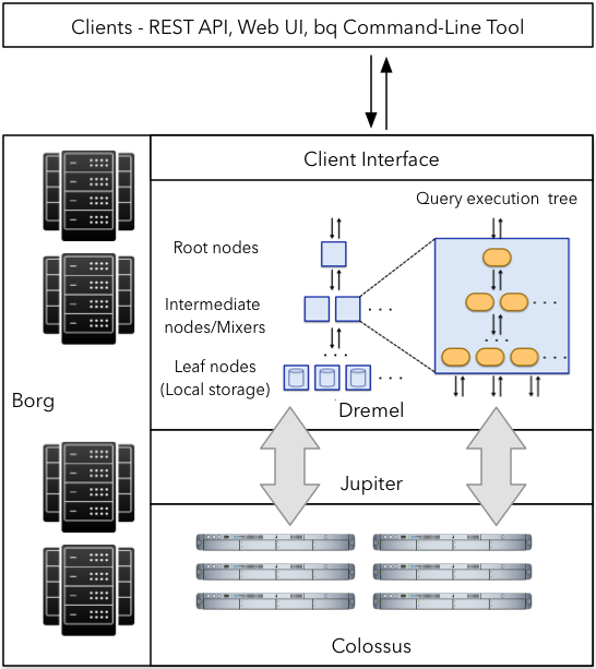
BigQuery and Dremel share the same basic architecture. By incorporating Dremel’s columnar storage and tree architecture, BigQuery offers unprecedented performance. But BigQuery is much more than a Dremel. Dremel is just a launch tool for BigQuery. BigQuery uses innovative Google technologies such as Borg, Colossus, Capacitor, and Jupiter.
A BigQuery client (typically the BigQuery web UI or bg command-line tool or REST API) communicates with the Dremel module through the client interface. Borg – Google’s massive cluster management system – allocates computing capacity for Dremel jobs. Dremel jobs read data from Google Colossus file systems using the Jupiter network, perform various SQL operations, and return results to the client. Dremel implements a multi-level service tree for query execution, described in more detail in the following sections.
It is important to note that the BigQuery architecture separates the concepts of storage (Colossus) and compute (Borg) and allows them to scale independently – an essential requirement for an elastic data warehouse. This makes BigQuery more economical and scalable compared to its counterparts.
Storage space
The most expensive part of any big data analytics platform is almost always disk I/O. BigQuery stores data in a columnar format known as a condenser. As you might expect, each BigQuery table field, i.e., column, is stored in a separate Capacitor file, which allows BigQuery to achieve a very high compression ratio and scan throughput. In 2016, Capacitor replaced the previous generation’s ColumnIO – optimised column storage format. Unlike ColumnIO Capacitor, BigQuery allowed BigQuery to directly work with compressed data without decompressing the data at runtime.
You can import data into the BigQuery repository using batch loading or streaming. BigQuery encodes each column separately into the Capacitor format during the import process. Once all column data is encoded, it is written back to Colossus. During encoding, various statistics about the data are collected, which are later used for query planning.
BigQuery uses Capacitor to store data in Colossus. Colossus is the latest generation of Google’s distributed file system and the successor to GFS (Google File Systems). Colossus handles cluster-wide replication, recovery, and distributed management. In addition, it provides client-controlled replication and encryption. When writing data to Colossus, BigQuery decides on an initial sharing strategy that evolves based on queries and access patterns. Once the data is written, BigQuery begins replicating the data across different data centers to enable the highest availability.
In summary, Capacitor and Colossus are critical components of the high-performance characteristics offered by BigQuery. Colossus allows data to be partitioned into multiple partitions, enabling lightning-fast parallel reads, while the capacitor reduces the demands on scan throughput. Together, they make it possible to process a terabyte of data per second.
Native & External
So far, we have discussed storage for a native BigQuery table. However, BigQuery can also query external data sources without importing data into native BigQuery tables. For example, BigQuery can perform direct queries against Google Cloud Bigtable, Google Cloud Storage, and Google Drive.
When using an external data source (aka federated data source), BigQuery loads the data into the Dremel engine on the fly. Generally, queries run against external data sources will be slower than native BigQuery tables. Query performance also depends on the type of external storage. For example, queries to Google Cloud Storage will perform better than Google Drive. Therefore, you should always import data into the table before running queries for performance.
Compute
BigQuery uses Borg for data processing. Borg runs thousands of Dremel jobs in one or more clusters of tens of thousands of machines. In addition to allocating computing power for Dremel jobs, Borg handles fault tolerance.
This image is taken from – radish.io
Network
In addition to disk I/O, network speed often limits large data loads. Because of the separation between the compute and storage layers, BigQuery requires an ultra-fast network that can deliver terabytes of data in seconds directly from storage to the add-to-run Dremel jobs. Google’s Jupiter network allows BigQuery to use one petabit/s of total bandwidth.
Read-only
Because of columnar storage, existing records cannot be updated, so BigQuery primarily supports read-only use cases. This means you can always write processed data back into new tables.
Design model
The Dremel engine uses a multi-level operator tree to scale
SQL queries. This tree architecture was specifically designed to run on commodity hardware. Dremel uses a query dispatcher that provides fault tolerance and schedules queries based on priority and load.
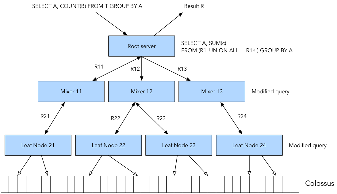
In the service tree, the root server receives incoming queries from clients and routes the queries to the next level. The root server is responsible for returning query results to the client. The leaf nodes of the service tree do the heavy lifting of reading data from Colossus and performing filters and partial aggregation. To parallelize a query, each provisioning tier (root and mixers) executes a rewrite of the query, and finally, the modified and split queries reach the end nodes for execution.
Few things happen while the query is being rewritten. First, the query is modified to include the table’s horizontal partitions, i.e., the shards (originally, the paper Dremel shards were referred to as tablets). Second, a specific SQL clause can be removed before sending to the end nodes. Finally, there are hundreds or thousands of leaf nodes in a typical Dremel tree. Leaf nodes return results to mixers or intermediate nodes. Mixers aggregate the results produced by the leaf nodes.
Each leaf node provides a thread of execution or several processing units, often called slots. It is important to note that BigQuery automatically calculates how many blocks should be assigned to each query. The number of allocated slots depends on the query’s size and complexity. At the time of writing, the on-demand pricing model allows a maximum of 2,000 concurrent slots per BigQuery project.
To help you understand how the Dremel motor works and how the operator tree is run, let’s look at a simple query,

When the root server receives this query, the first thing it does is translate the query into a form that can be handled by the next level of the service tree. First, it determines all fragments of table T and then simplifies the query.

In this case, R11, R12, . . . , R1n are the results of queries sent to Mixer 1, . . . , n at level 1 of the serving tree.
Next, Mixers will modify the incoming queries so that they can pass them to the leaf nodes. Leaf nodes receive customized queries and read data from Colossus shards. First, the Lead node reads the data for the columns or fields specified in the query. Then, as the leaf node scans the shards, it traverses the open column files in parallel, one row at a time.
The data between the leaf nodes can be shuffled depending on the queries. For example, when you use GROUP EACH BY in your queries, the Dremel engine will perform a shuffle operation. Therefore, it is important to understand the amount of mixing your queries require. Some queries with operations like JOIN can run slowly if you don’t optimize them to reduce mixing. Therefore, BigQuery recommends truncating the data as early as possible in the query so that the shuffling caused by your operations is applied to a limited data set.
Since BigQuery charges you for every 1 TB of data scanned by leaf nodes, we should avoid scanning too large or too often. There are many ways to do this. One of them is the division of tables by date. For each table, additional data sharing by BigQuery that you cannot control. Instead of using one big query, break them into small steps and store the query results in temporary tables for each step so that subsequent queries have fewer data to scan. It may sound counterintuitive, but the LIMIT clause does not reduce the amount of data scanned by the query. If you only need sample data to examine, you should use the Preview options and not a query with a LIMIT clause.
Different optimizations are applied at each level of the service tree so that nodes can return results as soon as they are ready to serve. This includes tricks like priority queue or streaming results.
This image is taken from – radish.io
Something from mathematics
Now that we understand the architecture of BigQuery, let’s take a look at how resources were allocated when running an interactive query using BigQuery. Let’s say you’re querying a 10-column table with 10 TB of storage and 1000 shards. As mentioned earlier, when you import data into a table, BigQuery determines the optimal number of fragments for your table and tunes them based on data access and query pattern. In addition, BigQuery creates condenser files for each table column during data import. In this particular case, 10 capacitor sets per shard.
There are actually 1000 x 10 files to read if you do a full scan (i.e., select * from the table). You have 2,000 concurrent slots to read those 10,000 files (if you’re using BigQuery’s on-demand pricing model and assuming it’s just an interactive query you’re running as part of a BigQuery project), on average, one slot will read 5 capacitor files or 5 GB of data. It takes anywhere from ~4 seconds (10 Gbps) to load that much data using the Jupiter network, which is one of the critical differentiators for BigQuery as a service.
We should avoid doing a full scan because a full scan is the most expensive – computationally and cost-wise – way to query your data. Instead, we should only query the columns we need; this is an essential best practice for any column-oriented database or data warehouse.
Data model
BigQuery stores data as nested relationships. A tree represents the schema for a session. Tree nodes are attributes, and leaf attributes contain values. BigQuery data is stored in columns (sheet attributes). In addition to the compressed column values, each column also holds structure information that indicates how the values in the column are distributed in the tree using two parameters – definition level and repetition. These parameters help reconstruct a full or partial representation of a record by reading only the required columns.
This image is taken from – radish.io
We should deformalize the data whenever possible to take full advantage of the nested and repeating fields that the BigQuery data structure offers. In addition, denormalization localizes the required data to individual nodes, reducing the network communication required for shuffling between slots.
Query language
BigQuery currently supports two different SQL dialects: standard SQL and legacy SQL. Standard SQL is compatible with SQL 2011 and offers several advantages over the older alternative. Legacy SQL is the original Dremel dialect. Both SQL dialects support user-defined functions (UDFs). You can write queries in any format, but Google recommends standard SQL. In 2014, Google published another paper describing how the Dremel engine uses a semi-flattened tree data structure and a standard SQL evaluation algorithm to support standard SQL query computation. This semi-flattened data structure is more aligned with the way Dremel processes data and is usually much more compact than flattened data
It’s important to note that when you deformalize data, you can preserve some relationships by using nested and repeating fields instead of fully merging the data. This is exactly what we will call a semi-flattening data structure.
Alternatives
Although there are several alternatives to BigQuery – both in the open-source domain and in the cloud as a service offering – it is still difficult to replicate the scale and performance of BigQuery. Mainly because Google does a great job of connecting infrastructure with BigQuery software. Open source solutions like Apache Drill and Presto require extensive infrastructure engineering and ongoing operational overhead to match BigQuery’s performance. Amazon Athena—a serverless interactive query service offered by Amazon Web Services (AWS)—is a hosted version of Presto with ANSI SQL support, but the service is relatively new. Nevertheless, initial benchmarks indicate that BigQuery still has a massive lead in terms of performance.
Conclusion
BigQuery is designed to query structured and semi-structured data using standard SQL. It is highly optimized for query performance and provides extremely high cost-efficiency. In addition, BigQuery is a cloud-based, fully managed service, meaning there is no operational overhead. As a result, it is better suited for interactive queries and OLAP/BI use cases. Google’s cloud infrastructure technologies, such as Borg, Colossus, and Jupiter, are a crucial differentiator for BigQuery outperforming some of its peers.
Till now, we have seen,
- BigQuery architecture helps implement various BigQuery best practices, including cost management, query performance optimization, and storage optimization.
- Capacitor and Colossus are critical components of the high-performance characteristics offered by BigQuery. BigQuery stores data as nested relationships. A tree represents the schema for a session. Tree nodes are attributes, and leaf attributes contain values.
- It’s important to note that when you deformalize data, you can preserve some relationships by using nested and repeating fields instead of fully merging the data. This is exactly what we will call a semi-flattening data structure.
The media shown in this article is not owned by Analytics Vidhya and is used at the Author’s discretion.