Introduction

In recent years, Graph Neural Networks (GNNs) have emerged as a potent tool for analyzing and understanding graph-structured data. By leveraging the inherent structure and relationships within graphs, GNNs offer a unique approach to solving a wide range of machine learning tasks. In this blog, we will explore this concept from theory to GNN Implementation. From fundamental principles to advanced concepts, we will cover everything necessary to understand and effectively apply GNNs.

Learning Objective

• Understand GNNs’ role in analyzing graph data.
• Explore node classification, link prediction, and graph generation.
• Define types like directed vs. undirected and weighted vs. unweighted.
• Create and visualize graphs using Python libraries.
• Learn about its significance in GNNs for node communication.
• Explore GCNs, GATs, and graph pooling for efficient graph analysis.

This article was published as a part of the Data Science Blogathon.

Why are GNNs Important?

Traditional machine learning models, such as convolutional neural networks (CNNs) and recurrent neural networks (RNNs), are designed to operate on grid-like data structures. However, many real-world datasets, such as social networks, citation networks, and biological networks, exhibit a more complex structure represented by graphs. This is where GNNs shine. They are specifically tailored to handle graph-structured data, making them well-suited for a variety of applications.

Practical Applications of GNN

Throughout this blog, we will explore several practical applications of GNNs across different domains. Some of the applications we will cover include:

1. Node Classification: Predicting properties or labels associated with individual nodes in a graph, such as classifying users in a social network based on their interests.
2. Link Prediction: Anticipating missing or future connections between nodes in a graph, such as predicting potential interactions between proteins in a biological network.
3. Graph Classification: Classifying entire graphs based on their structural properties, such as categorizing molecular graphs by their chemical properties.
4. Graph Generation: Generating new graphs that exhibit similar properties to a given set of input graphs, such as creating realistic social networks or molecular structures.

Definition of Graphs

In mathematics and computer science, a graph is a data structure composed of nodes (also known as vertices) and edges (also known as links or connections) that establish relationships between the nodes. Graphs are widely used to model and analyze relationships between entities in various real-world scenarios

Types of Graphs

Graphs can be classified into several types based on different characteristics:

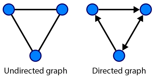
Directed vs. Undirected Graphs

In a directed graph, edges have a direction associated with them, indicating a one-way relationship between nodes. In contrast, undirected graphs have edges without any specific direction, representing mutual relationships between nodes.

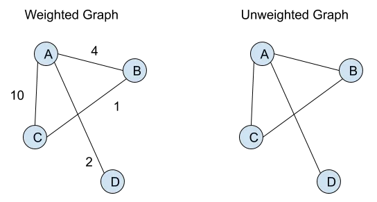
Weighted vs. Unweighted Graphs

In a weighted graph, each edge is assigned a numerical value (weight) that represents the strength or cost of the relationship between nodes. Unweighted graphs, on the other hand, do not have such values associated with edges.

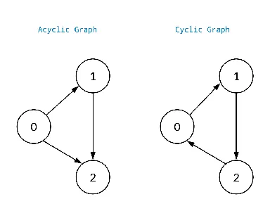
Cyclic vs. Acyclic Graphs

A cyclic graph contains at least one cycle, i.e., a sequence of edges that form a closed loop. In contrast, an acyclic graph does not contain any cycles.

Example Dataset: Social Network Graph

As an example dataset for hands-on exploration, let’s consider a social network graph representing friendships between users. In this graph:

• Nodes represent individual users.
• Undirected edges represent friendships between users.
• Each node may have associated attributes such as user IDs, names, or interests.

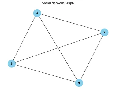
Here’s a simplified representation of a social network graph:

Nodes (Users):     Edges (Friendships):
1 (Alice)          (1, 2), (1, 3), (1, 4)
2 (Bob)            (2, 3), (2, 4)
3 (Charlie)        (3, 4)
4 (David)

In this graph:

• Alice is friends with Bob, Charlie, and David.
• Bob is friends with Charlie and David.
• Charlie is friends with David.
• David has no additional friends in this network.

Now, let’s look into a practical hands-on exploration of the social network graph using Python and the NetworkX library.

import networkx as nx
import matplotlib.pyplot as plt

# Create an empty undirected graph
social_network = nx.Graph()

# Add nodes representing users
users = [1, 2, 3, 4]
social_network.add_nodes_from(users)

# Add edges representing friendships
friendships = [(1, 2), (1, 3), (1, 4), (2, 3), (2, 4), (3, 4)]
social_network.add_edges_from(friendships)

# Visualize the social network graph
pos = nx.spring_layout(social_network)  # Positions for all nodes
nx.draw(social_network, pos, with_labels=True, node_color='skyblue', node_size=1000,
font_size=12, font_weight='bold')
plt.title("Social Network Graph")
plt.show()

In the code above:

• We first import the NetworkX library, which provides tools for working with graphs.
• We create an empty undirected graph named social_network.
• We add nodes representing individual users using their unique IDs.
• We add edges representing friendships between users based on the provided list of friendships.
• Finally, we visualize the social network graph using the nx.draw() function, specifying node positions, labels, colors, and other visual attributes.

Interpreting the Social Network Graph

In the visual representation of the social network graph, each node corresponds to a user, and each edge represents a friendship between users. By examining the graph, we can infer various insights:

1. Node Representation: Each node is labeled with a unique user ID, allowing us to identify individual users within the network.
2. Edge Representation: Edges connecting nodes indicate mutual friendships between users. For example, if there is an edge between nodes 1 and 2, it means that user 1 and user 2 are friends.
3. Network Structure: By observing the overall structure of the graph, we can identify clusters of users who are interconnected through mutual friendships.

Beyond visual inspection, we can perform additional analysis and exploration on the social network graph using NetworkX and other Python libraries. Here are some examples of what you can do:

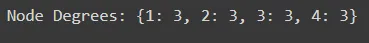
Node Degree

Calculate the degree of each node, which represents the number of friendships associated with that user.

# Calculate node degrees
node_degrees = dict(social_network.degree())
print("Node Degrees:", node_degrees)

Connected Components

Identify connected components within the graph, representing groups of users who are mutually connected through friendships.

# Find connected components
connected_components = list(nx.connected_components(social_network))
print("Connected Components:", connected_components)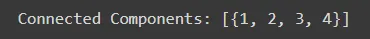

 Shortest Paths

Find the shortest path between two users, indicating the minimum number of friendships required to connect them.

# Find shortest path between two users
shortest_path = nx.shortest_path(social_network, source=1, target=4)
print("Shortest Path from User 1 to User 4:", shortest_path)

Limitations of Traditional Machine Learning Approaches with Graph Data

Traditional machine learning approaches, such as convolutional neural networks (CNNs) and recurrent neural networks (RNNs), are designed to operate effectively on grid-like data structures, such as images, sequences, and tabular data. However, these approaches face significant limitations when applied to graph-structured data:

1. Permutation Invariance: Traditional models lack permutation invariance, meaning they treat inputs as fixed-size vectors or sequences without considering the inherent permutation of nodes in a graph. As a result, they struggle to effectively capture the complex relationships and dependencies within graphs.
2. Variable-Sized Inputs: Graphs can have varying numbers of nodes and edges, making it challenging to process them using fixed-size architectures. Traditional models often require preprocessing techniques, such as graph discretization or graph embedding, which may lead to information loss or computational inefficiency.
3. Local vs. Global Information: Traditional models typically focus on capturing local information within neighborhoods or sequences, but they may struggle to incorporate global information that spans the entire graph. This limitation can hinder their ability to make accurate predictions or classifications based on the holistic structure of the graph.
4. Graph-Dependent Structure: Graph-structured data exhibits a rich, interconnected structure with heterogeneous node and edge attributes. Traditional models are not inherently equipped to handle this complex structure, leading to suboptimal performance and generalization on graph-related tasks.

Introducing Graph Neural Networks (GNNs) as a Solution

Graph Neural Networks (GNNs) offer a powerful solution to overcome the limitations of traditional machine learning approaches when working with graph-structured data. GNNs extend neural network architectures to directly operate on graph-structured inputs, enabling them to effectively capture and process information from nodes and edges within the graph.

Key features and advantages of GNNs include:

1. Graph Representation Learning: GNNs learn distributed representations (embeddings) for nodes and edges in the graph, allowing them to encode both structural and attribute information within a unified framework.
2. Message Passing: GNNs leverage message passing algorithms to propagate information between neighboring nodes in the graph. By iteratively aggregating and updating node representations based on local neighborhood information, GNNs can capture complex dependencies and relational patterns within the graph.
3. Permutation Invariance: GNNs inherently account for the permutation of nodes within a graph, ensuring that they operate consistently regardless of node ordering. This property enables GNNs to maintain spatial awareness and effectively model graph-structured data without the need for explicit preprocessing.
4. Scalability and Flexibility: GNNs are highly scalable and flexible, capable of handling graphs of varying sizes and structures. They can be adapted to different types of graph-related tasks, including node classification, link prediction, graph classification, and graph generation.

Fundamentals of Graph Neural Networks

Graph Representation

Graph representation is a fundamental aspect of Graph Neural Networks (GNNs), as it involves encoding the structure and attributes of a graph into a format suitable for computational processing. In this section, we will explore how to represent graphs using popular libraries such as NetworkX and PyTorch Geometric, along with code snippets for creating and visualizing graphs.

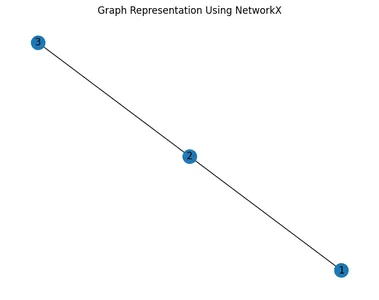
Representation Using NetworkX

NetworkX is a Python library for creating, manipulating, and studying complex networks, including graphs. It provides a convenient interface for building graphs and performing various graph operations.

import networkx as nx
import matplotlib.pyplot as plt

# Create an empty undirected graph
G = nx.Graph()

# Add nodes
G.add_node(1)
G.add_node(2)
G.add_node(3)

# Add edges
G.add_edge(1, 2)
G.add_edge(2, 3)

# Visualize the graph
nx.draw(G, with_labels=True)
plt.title("Graph Representation Using NetworkX")
plt.show()

Representation Using PyTorch Geometric

PyTorch Geometric is a library for deep learning on irregular input data, such as graphs, with support for efficient batching and GPU acceleration.

# install torch-geometric 
!pip install torch-geometric -f https://pytorch-geometric.com/whl/torch-1.9.0+cu111.html

# import libraries
import torch
from torch_geometric.data import Data
from torch_geometric.utils import to_networkx
import matplotlib.pyplot as plt
import networkx as nx

# Define edge indices and node features
edge_index = torch.tensor([[0, 1], [1, 2]], dtype=torch.long)
x = torch.tensor([[1], [2], [3]], dtype=torch.float)

# Create a PyTorch Geometric Data object
data = Data(x=x, edge_index=edge_index.t().contiguous())

# Convert to NetworkX graph
G = to_networkx(data)

# Visualize the graph
nx.draw(G, with_labels=True)
plt.title("Graph Representation Using PyTorch Geometric")
plt.show()

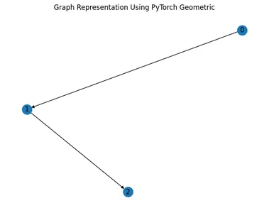
In both examples, we’ve created a simple graphs with three nodes and two edges. However, the methods of graph representation differ slightly between NetworkX and PyTorch Geometric.

NetworkX Representation

• In NetworkX, nodes and edges are added individually using add_node() and add_edge() methods.
• The visualization of the graph is straightforward, with nodes represented as circles and edges as lines connecting them.

PyTorch Geometric Representation

• PyTorch Geometric represents graphs using specialized data structures tailored for deep learning tasks.
• Node features and edge connectivity are encapsulated within a Data object, providing a more structured representation.
• PyTorch Geometric integrates seamlessly with PyTorch, making it suitable for graph-based deep learning tasks.

Interpretation

• Both representations serve their respective purposes, NetworkX is well-suited for graph analysis and visualization tasks, while PyTorch Geometric provides a framework for deep learning on graphs.
• Depending on the task at hand, you can choose the appropriate representation and library. For traditional graph algorithms and visualization, NetworkX may be preferable. For deep learning tasks involving graphs, PyTorch Geometric offers more flexibility and efficiency.

Message Passing

In Graph Neural Networks (GNNs), message passing is a fundamental concept that allows nodes in a graph to communicate with each other. Think of it like passing notes in class – each node sends a message to its neighbors, and then they all update their information based on these messages.

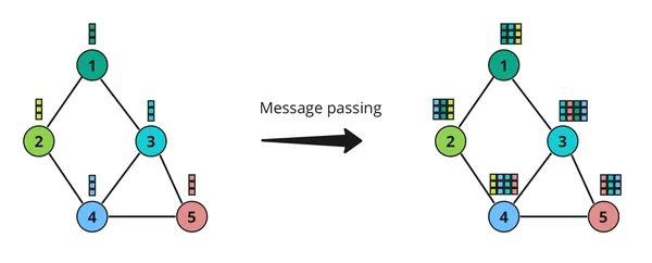
Here’s How it Works

1. Sending Messages: Each node gathers information from its neighbors and sends out a message. This message typically contains information about the node itself and its neighbors.
2. Receiving Messages: Once a node receives messages from its neighbors, it combines this information with its own and updates its internal representation. This step helps the node understand its place in the larger graph.
3. Updating Information: After receiving messages from neighbors, each node updates its own information based on these messages. This update process ensures that each node has a more complete understanding of the graph’s structure and properties.

Message passing is crucial in GNNs because it allows nodes to leverage information from their local neighborhoods to make informed decisions. It’s like neighbors sharing gossip – by exchanging messages, nodes can collectively gain insights into the overall structure and dynamics of the graph. This enables GNNs to perform tasks such as node classification, link prediction, and graph classification effectively.

Implementing Message Passing in Python

To implement a simple message passing algorithm in Python, we’ll create a basic Graph Neural Network (GNN) layer that performs message passing between neighboring nodes and updates node representations. Let’s use a toy graph with randomly initialized node features and adjacency matrix for demonstration purposes.

import numpy as np

# Define a toy graph with 4 nodes and their initial features
num_nodes = 4
num_features = 2
adjacency_matrix = np.array([[0, 1, 0, 1],
                             [1, 0, 1, 1],
                             [0, 1, 0, 0],
                             [1, 1, 0, 0]])  # Adjacency matrix

node_features = np.random.rand(num_nodes, num_features)  # Random node features

# Define a simple message passing function
def message_passing(adj_matrix, node_feats):
    updated_feats = np.zeros_like(node_feats)
    num_nodes = len(node_feats)
    
    # Iterate over each node
    for i in range(num_nodes):
        # Gather neighboring nodes based on adjacency matrix
        neighbors = np.where(adj_matrix[i] == 1)[0]
        
        # Aggregate messages from neighbors
        message = np.sum(node_feats[neighbors], axis=0)
        
        # Update node representation
        updated_feats[i] = node_feats[i] + message
    
    return updated_feats

# Perform message passing for one iteration
updated_features = message_passing(adjacency_matrix, node_features)
print("Updated Node Features after Message Passing:")
print(updated_features)

# output
#Updated Node Features after Message Passing:
#[[0.5602586  1.54137027]
# [0.61232074 1.59538215]
# [0.28878133 0.69739586]
#[0.5602586  1.54137027]]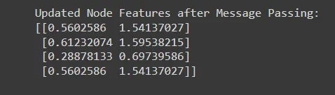

In this code:

• We define a toy graph with 4 nodes and their initial features, represented by a random matrix for node features and an adjacency matrix for edges.
• We create a simple message passing function (message_passing) that iterates over each node, gathers messages from neighboring nodes based on the adjacency matrix, and updates node representations by aggregating messages.
• We perform one iteration of message passing on the toy graph and print the updated node features.
• The message_passing function iterates over each node in the graph and gathers messages from its neighboring nodes.
• The neighbors variable stores the indices of neighboring nodes based on the adjacency matrix.
• The message variable aggregates node features from neighboring nodes.
• The node representation is updated by adding the message to the original node features.
• This process is repeated for each node, resulting in updated node representations after one iteration of message passing.

Extending Message Passing for Complex Relationships

Let’s extend the example to perform multiple iterations of message passing to capture more complex relationships within the graph.

# Define the number of message passing iterations
num_iterations = 3

# Perform multiple iterations of message passing
for _ in range(num_iterations):
    node_features = message_passing(adjacency_matrix, node_features)

print("Updated Node Features after Multiple Iterations of Message Passing:")
print(node_features)

# output
# Updated Node Features after Multiple Iterations of Message Passing:
#[[ 5.48729515 14.73176393]
# [ 6.38839722 17.02454194]
# [ 2.92272134  7.66829656]
# [ 5.48729515 14.73176393]]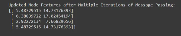

• By performing multiple iterations of message passing, we allow information to propagate and accumulate across the graph, capturing increasingly complex relationships and dependencies.
• Each iteration refines the node representations based on information aggregated from neighboring nodes, leading to progressively enhanced node embeddings.

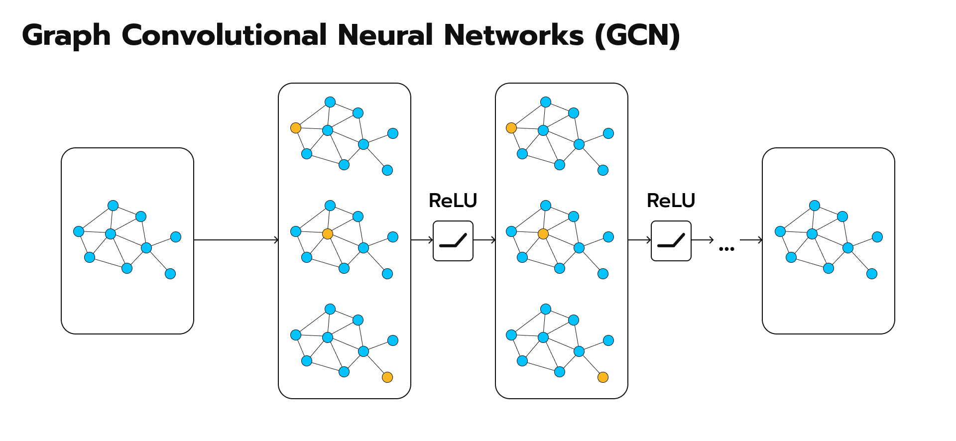
Graph Convolutional Networks (GCNs)

Graph Convolutional Networks (GCNs), the superheroes of the machine learning world, equipped with the superpower to navigate and extract insights from these tangled webs. GCNs are not just another algorithm; they’re a revolutionary approach that revolutionizes how we analyze and understand graph-structured data. In Graph Neural Networks (GNNs), Graph Convolutional Networks (GCNs) are a specific type of model designed to operate on graph-structured data. GCNs are inspired by convolutional neural networks (CNNs) used in image processing, but adapted to handle the irregular and non-Euclidean structure of graphs.

Here’s a simplified explanation

• Understanding Graphs: In many real-world scenarios, data can be represented as a graph, where entities (nodes) are connected by relationships (edges). For example, in a social network, people are nodes, and friendships are edges.
• What GCNs Do: GCNs aim to learn useful representations of nodes in a graph by taking into account the features of neighboring nodes. They do this by propagating information through the graph using a process called message passing.
• Message Passing: At each layer of a GCN, nodes aggregate information from their neighbors, typically by taking a weighted sum of their features. This aggregation process is akin to a node gathering information from its immediate surroundings.
• Learning Representations: Through multiple layers of message passing, GCNs learn increasingly abstract representations of nodes that capture both local and global graph structures. These representations can then be used for various downstream tasks, such as node classification, link prediction, or graph classification.
• Training: Like other neural networks, GCNs are trained using labeled data, where the model learns to predict node labels or other properties of interest based on input graph data.

GCNs are powerful tools for learning from graph-structured data, enabling tasks such as node classification, link prediction, and graph-level prediction in a variety of domains, including social networks, biological networks, and recommendation systems.

Example of a GCN Model

Let’s define a simple GCN model with two graph convolutional layers to understand better.

import time
import torch
import torch.nn.functional as F
import torch_geometric.transforms as T
from torch_geometric.datasets import Planetoid
from torch_geometric.nn import GCNConv


if torch.cuda.is_available():
    device = torch.device('cuda')
elif hasattr(torch.backends, 'mps') and torch.backends.mps.is_available():
    device = torch.device('mps')
else:
    device = torch.device('cpu')


class GCN(torch.nn.Module):
    def __init__(self, in_channels, hidden_channels, out_channels):
        super().__init__()
        self.conv1 = GCNConv(in_channels, hidden_channels)
        self.conv2 = GCNConv(hidden_channels, out_channels)

    def forward(self, x, edge_index, edge_weight=None):
        x = F.dropout(x, p=0.5, training=self.training)
        x = self.conv1(x, edge_index, edge_weight).relu()
        x = F.dropout(x, p=0.5, training=self.training)
        x = self.conv2(x, edge_index, edge_weight)
        return x

We’ll use the Cora dataset, a citation network. PyTorch Geometric provides built-in functions to download and preprocess popular datasets.

#dataset

dataset = Planetoid(root='data', name='Cora', transform=T.NormalizeFeatures())
data = dataset[0].to(device)


transform = T.GDC(
    self_loop_weight=1,
    normalization_in='sym',
    normalization_out='col',
    diffusion_kwargs=dict(method='ppr', alpha=0.05),
    sparsification_kwargs=dict(method='topk', k=128, dim=0),
    exact=True,
)
data = transform(data)

We’ll train the GCN model on the Cora dataset using standard training procedures.

model = GCN(
    in_channels=dataset.num_features,
    hidden_channels=16,
    out_channels=dataset.num_classes,
).to(device)

optimizer = torch.optim.Adam([
    dict(params=model.conv1.parameters(), weight_decay=5e-4),
    dict(params=model.conv2.parameters(), weight_decay=0)
], lr=0.01)  # Only perform weight-decay on first convolution.


def train():
    model.train()
    optimizer.zero_grad()
    out = model(data.x, data.edge_index, data.edge_attr)
    loss = F.cross_entropy(out[data.train_mask], data.y[data.train_mask])
    loss.backward()
    optimizer.step()
    return float(loss)
    
@torch.no_grad()
def test():
    model.eval()
    pred = model(data.x, data.edge_index, data.edge_attr).argmax(dim=-1)

    accs = []
    for mask in [data.train_mask, data.val_mask, data.test_mask]:
        accs.append(int((pred[mask] == data.y[mask]).sum()) / int(mask.sum()))
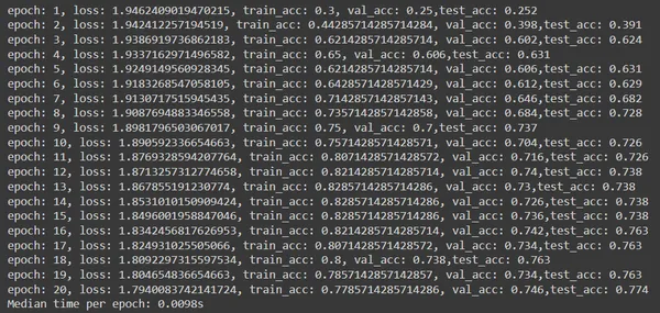
    return accs

Training till 20 epochs

best_val_acc = test_acc = 0
times = []
for epoch in range(1, 20 + 1):
    start = time.time()
    loss = train()
    train_acc, val_acc, tmp_test_acc = test()
    if val_acc > best_val_acc:
        best_val_acc = val_acc
        test_acc = tmp_test_acc
    print(f"epoch: {epoch}, loss: {loss}, train_acc: {train_acc}, val_acc: {val_acc},
    test_acc: {test_acc}")
    times.append(time.time() - start)
print(f'Median time per epoch: {torch.tensor(times).median():.4f}s')

Explanation

• The code begins by importing necessary libraries including time, torch, torch.nn.functional (often imported as F), and components from torch_geometric including transforms, datasets, and neural network modules.
• It checks if CUDA is available for GPU computation; if not, it checks for the availability of the Multi-Process Service (MPS). If neither is available, it defaults to CPU.
• The code loads the Cora dataset from the Planetoid dataset collection in PyTorch Geometric. It normalizes the features and loads the dataset onto the specified device (CPU or GPU).
• It applies a Graph Diffusion Convolution (GDC) transformation to the dataset. GDC is a pre-processing step that enhances the representation of the graph structure.
• A Graph Convolutional Network (GCN) model is defined using PyTorch’s torch.nn.Module class. It consists of two GCN layers (GCNConv) followed by ReLU activation and dropout layers.
• An Adam optimizer is defined to optimize the parameters of the GCN model. Weight decay is applied to the parameters of the first convolutional layer only.
• The train function is defined to train the GCN model. It sets the model to training mode, computes the output, calculates the loss using cross-entropy, performs backpropagation, and updates the parameters using the optimizer.
• The test function evaluates the trained model on the training, validation, and test sets. It computes predictions, calculates accuracy for each set, and returns the accuracies.
• The code iterates through 20 epochs, calling the train function to train the model and the test function to evaluate it on the validation and test sets. It also tracks the best validation accuracy and corresponding test accuracy.
• The results including epoch number, loss, training accuracy, validation accuracy, and test accuracy are printed for each epoch. Also, the median time taken per epoch is computed and printed at the end of training.

Graph Attention Networks (GATs)

Graph Attention Networks (GATs) are a type of Graph Neural Network (GNN) architecture that introduces attention mechanisms to learn node representations in a graph. Attention mechanisms have been widely successful in natural language processing tasks, allowing models to focus on relevant parts of input sequences. GATs extend this idea to graphs, enabling the model to dynamically weigh the importance of neighboring nodes’ features when aggregating information.

The key idea behind GATs is to compute attention scores between a central node and its neighbors, which are then used to compute weighted feature representations of the neighbors. These weighted representations are aggregated to produce an updated representation of the central node. By learning these attention scores during training, GATs can effectively capture the importance of different neighbors for each node in the graph.

One of the main advantages of GATs is their ability to capture complex relationships and dependencies between nodes in the graph. Unlike traditional GNN architectures that use fixed aggregation functions, GATs can adaptively assign higher weights to more relevant neighbors, leading to more expressive node representations.

Here’s a breakdown of GATs

• Attention Mechanisms: Inspired by the attention mechanism commonly used in natural language processing, GATs assign different attention scores to each neighbor of a node. This allows the model to focus on more relevant neighbors while aggregating information.
• Learning Weights: Instead of using fixed weights for aggregating neighbors’ features, GATs learn these weights dynamically during training. This means that the model can adaptively assign higher importance to nodes that are more relevant to the current task.
• Multi-Head Attention: GATs often employ multiple attention heads, each learning a different set of weights. This enables the model to capture different aspects of the relationships between nodes and helps improve performance.
• Representation Learning: Like other GNNs, GATs aim to learn meaningful representations of nodes in a graph. By leveraging attention mechanisms, GATs can capture complex patterns and dependencies in the graph structure, leading to more expressive node embeddings.

Example of a GAT Model

Let’s create a GAT-based model architecture using the defined Graph Attention Layer.

import time
import torch
import torch.nn.functional as F
import torch_geometric.transforms as T
from torch_geometric.datasets import Planetoid
from torch_geometric.nn import GATConv

device = torch.device('cuda' if torch.cuda.is_available() else 'cpu')

class GAT(torch.nn.Module):
    def __init__(self, in_channels, hidden_channels, out_channels, heads):
        super().__init__()
        self.conv1 = GATConv(in_channels, hidden_channels, heads, dropout=0.6)
        # On the Pubmed dataset, use `heads` output heads in `conv2`.
        self.conv2 = GATConv(hidden_channels * heads, out_channels, heads=1,
                             concat=False, dropout=0.6)

    def forward(self, x, edge_index):
        x = F.dropout(x, p=0.6, training=self.training)
        x = F.elu(self.conv1(x, edge_index))
        x = F.dropout(x, p=0.6, training=self.training)
        x = self.conv2(x, edge_index)
        return x

We’ll again use the Cora dataset.

dataset = Planetoid(root='data', name='Cora', transform=T.NormalizeFeatures())
data = dataset[0].to(device)

hidden_channels=8
heads=8
lr=0.005
epochs=10

model = GAT(dataset.num_features, hidden_channels, dataset.num_classes,
            heads).to(device)
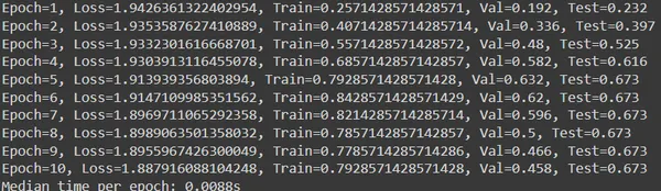
optimizer = torch.optim.Adam(model.parameters(), lr=0.005, weight_decay=5e-4)

Training GAT till 10 epochs

def train():
    model.train()
    optimizer.zero_grad()
    out = model(data.x, data.edge_index)
    loss = F.cross_entropy(out[data.train_mask], data.y[data.train_mask])
    loss.backward()
    optimizer.step()
    return float(loss)


@torch.no_grad()
def test():
    model.eval()
    pred = model(data.x, data.edge_index).argmax(dim=-1)

    accs = []
    for mask in [data.train_mask, data.val_mask, data.test_mask]:
        accs.append(int((pred[mask] == data.y[mask]).sum()) / int(mask.sum()))
    return accs


times = []
best_val_acc = final_test_acc = 0
for epoch in range(1, epochs + 1):
    start = time.time()
    loss = train()
    train_acc, val_acc, tmp_test_acc = test()
    if val_acc > best_val_acc:
        best_val_acc = val_acc
        test_acc = tmp_test_acc
    print(f"Epoch={epoch}, Loss={loss}, Train={train_acc}, Val={val_acc}, Test={test_acc}")
    times.append(time.time() - start)
print(f"Median time per epoch: {torch.tensor(times).median():.4f}s")

Code Explanation:

• Import necessary libraries: time, torch, torch.nn.functional (F), torch_geometric.transforms (T), torch_geometric.datasets.Planetoid, and torch_geometric.nn.GATConv, tailored for graph attention networks.
• Check for CUDA availability; set device to ‘cuda’ if available, else default to ‘cpu’.
• Define GAT model as a torch.nn.Module subclass. Initialize model’s layers, including two GATConv layers. Forward method passes input features (x) and edge indices through GATConv layers.
• Load Cora dataset using Planetoid class. Normalize dataset using T.NormalizeFeatures() and move it to selected device.
• Set hyperparameters: hidden_channels, heads, learning rate (lr), and epochs.
• Create GAT model instance with specified parameters, move it to selected device. Use Adam optimizer with specified lr and weight decay.
• Define train() and test() functions for model training and evaluation. train() performs a single iteration, calculates loss with cross-entropy, and updates parameters using backpropagation. test() evaluates model accuracy on training, validation, and test sets.
• Iterate over epochs, train model, and evaluate performance on validation set. Update best validation and corresponding test accuracy if new best is found. Print training and validation metrics for each epoch.
• Calculate and print median time per epoch at training end to measure speed.

Graph Pooling and Graph Classification

Graph Pooling and Graph Classification are essential components and tasks in Graph Neural Networks (GNNs) for handling graph-structured data. I won’t go into much details but let’s break down these concepts:

Graph Pooling

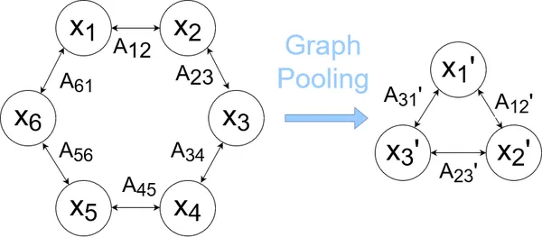
Graph pooling is a technique used to down sample or reduce the size of a graph while preserving its important structural and relational information. It is analogous to pooling layers in convolutional neural networks (CNNs) used for image data.

Pooling is employed to aggregate information from groups of nodes and edges in the graph, reducing computational complexity and enhancing the model’s ability to learn hierarchical representations. There are various graph pooling methods, including graph coarsening, hierarchical clustering, and attention-based pooling. These methods aim to retain important graph structures and features while discarding less relevant information.

Example

In a hierarchical pooling approach, the graph is recursively coarsened by merging nodes or aggregating neighborhoods until a desired size or level of abstraction is reached. This process enables the model to capture both local and global graph structures efficiently.

Graph Classification

Graph classification is a task in which an entire graph is assigned a single label or category based on its structural and feature information. It is a fundamental problem in graph analytics and has applications in various domains such as bioinformatics, social network analysis, and cheminformatics. 

The goal of graph classification is to learn discriminative representations of graphs that capture their inherent properties and characteristics, enabling accurate prediction of their labels. Graph classification methods typically involve extracting meaningful features from graphs using techniques such as graph embedding, graph neural networks, or graph kernels. These features are then fed into a classifier (e.g., a fully connected neural network or a support vector machine) to predict the graph labels.

Example

In a molecular graph classification task, each graph represents a molecule, and the task is to predict the molecule’s bioactivity or drug-likeness based on its chemical structure. Graph neural networks can be used to learn representations of molecules from their graph structures and atom features, which are then used for classification.

So, in summary, graph pooling techniques enable efficient down sampling of graphs while preserving important structural information, while graph classification methods aim to learn representations of entire graphs for accurate prediction of their labels. These components play crucial roles in enabling GNNs to handle graph-structured data effectively and perform various tasks such as node classification, link prediction, and graph classification across diverse domains.

Applications of GNNs

Graph Neural Networks (GNNs) have found applications across various domains due to their ability to model complex relationships and dependencies in data represented as graphs. Some examples of applying GNNs in real-world scenarios are:-

• Fraud Detection: Fraud detection is a critical task in various industries such as finance, insurance, and e-commerce. GNNs can be applied to detect fraudulent activities by modeling the relationships between entities (e.g., users, transactions) in a graph.
• Recommendation Systems: Recommendation systems aim to predict users’ preferences or interests in items (e.g., movies, products) based on their interactions. GNNs can capture the complex relationships between users and items in a graph to generate accurate recommendations.
• Drug Discovery: In drug discovery, GNNs can model the molecular structure of compounds and predict their properties or interactions with biological targets. This enables more efficient drug screening and lead optimization processes.

Challenges in Implementing and Scaling GNNs

• Graph Size: Scaling GNNs to large graphs with millions of nodes and edges poses computational challenges.
• Heterogeneous Data: Handling graphs with heterogeneous node and edge attributes requires specialized techniques.
• Interpretability: Interpreting the predictions of GNNs and understanding the learned representations remain challenging.

Conclusion

Graph Neural Networks (GNNs) have emerged as powerful tools for modeling and analyzing graph-structured data across various domains. From fraud detection and recommendation systems to drug discovery, GNNs offer versatile solutions to complex problems. Despite challenges, ongoing research and advancements continue to expand the capabilities and applications of GNNs, making them indispensable tools for data scientists and researchers alike. By understanding the principles and applications of GNNs, practitioners can leverage these techniques to address real-world challenges effectively.

Key Takeaways

• GNNs offer a powerful framework for analysing and learning from graph-structured data.
• They are applicable in various real-world scenarios such as social network analysis, recommendation systems, fraud detection, and drug discovery.
• Understanding the fundamentals of GNNs, including graph representation, message passing, and graph convolutional networks (GCNs), is crucial for effective implementation.
• Advanced concepts like Graph Attention Networks (GATs), and graph pooling techniques further enhance the capabilities of GNNs in capturing complex patterns in graphs.
• Practical examples and code snippets demonstrate how to apply GNNs to solve real-world problems, showcasing their effectiveness and practical utility.
• Challenges in implementing and scaling GNNs exist, but ongoing research focuses on addressing these challenges and improving the scalability and interpretability of GNNs.
• Readers are encouraged to explore further and experiment with GNNs in their own projects, leveraging available resources and documentation to drive innovation and address practical challenges.

Frequently Asked Questions

References

• PyTorch Geometric Github Repo
• PyTorch Geometric Documentation

The media shown in this article is not owned by Analytics Vidhya and is used at the Author’s discretion.