Comprehensive Guide on Non Parametric Tests
Introduction
In this article, we will explore what is hypothesis testing, focusing on the formulation of null and alternative hypotheses, setting up hypothesis tests and we will deep dive into parametric and non-parametric tests, discussing their respective assumptions and implementation in python. But our main focus will be on non-parametric tests like the Mann-Whitney U test and the Kruskal-Wallis test. By the end, you will have a comprehensive understanding of hypothesis testing and the practical tools to apply these concepts in your own statistical analyses.
Learning Objectives
- Understand the principles of hypothesis testing, including the formulation of null and alternative hypotheses.
- Setting up Hypothesis Test.
- Understanding about Parametric Test and its types.
- Understanding about Non Parametric Test and its types along with its implementations.
- Difference between Parametric and Non Parametric.
Table of contents
What is Hypothesis Testing ?
Hypothesis is a claim made by a person /organization. The claim is usually about population parameters such as mean or proportion and we seek evidence from a sample for the support of the claim.
Hypothesis testing, sometimes referred to as significance testing, is a method for confirming a claim or hypothesis about a parameter in a population using data measured in a sample. Using this method, we explore several theories by determining the potentiality that, had the population parameter hypothesis been true, a sample statistic might have been selected.
Hypothesis testing involves formulation of two hypotheses:
- Null hypothesis (H0)
- Alternative hypothesis (H1)
Null hypothesis : It is usually a hypothesis of no difference and usually denoted by H0. According to R.A Fisher , null hypothesis is the hypothesis which is tested for possible rejection under the assumption that it is true (Ref Fundamentals of Mathematical Statistics).
Alternative hypothesis: Any hypothesis which is complementary to the null hypothesis is called an alternative hypothesis, usually denoted by H1.
The objective of hypothesis testing is to either reject or retain a null hypothesis to establish a statistically significant relationship between two variables (usually one independent and one dependent variable, i.e. usually one is the cause and one is the effect) .
Setting up Hypothesis Test
- Describe the hypothesis in words or make a claim.
- Based on claim define null and alternative hypotheses.
- Identify the type of hypothesis test appropriate for the above claim.
- Identify the test statistics to be used for testing the validity of the null hypothesis.
- Decide the criteria for rejection and retention of null hypothesis. This is called significance value traditionally denoted by symbol α (alpha).
- Calculate the p-value which is the conditional probability of observing the test statistic value when the null hypothesis is true. In simple terms, p-value is the evidence in support of the null hypothesis.
Parametric and Non parametric test
Non-parametric statistical tests do not rely on assumptions about the parameters of the population distributions from which the data are sampled, whereas parametric statistical tests do.
Parametric Tests
Most statistical tests are performed using a set of assumptions as their foundation. The analysis may yield misleading or completely false conclusions when certain assumptions are violated.
Typically the assumptions are:
- Normality: The sampling distribution of parameters to be tested follows a normal (or at least symmetric) distribution.
- Homogeneity of variances: The variance of the data is the same across different groups unless we are testing for population means coming from two different populations.
Some of the parametric test are :
- Z-test : Test for population mean or variance or proportion when the population standard deviation is known.
- Student’s t-test: Test for population mean or variance or proportion when the population standard deviation is not known.
- Paired t-test: Used to compare the means of two related groups or conditions.
- Analysis of Variance (ANOVA): Used to compare means across three or more independent groups.
- Regression analysis: Used to assess the relationship between one or more independent variables and a dependent variable.
- Analysis of Covariance (ANCOVA): Extends ANOVA by incorporating additional covariates into the analysis.
- Multivariate Analysis of Variance (MANOVA): Extends ANOVA to assess differences in multiple dependent variables across groups.
Now let’s deep dive into Non parametric test.
Non parametric test
For the first time, Wolfowitz used the term “non-parametric” in 1942. To understand the idea of nonparametric statistics, one must first have a basic understanding of parametric statistics, which we have just discussed. A parametric test requires a sample that follows a specific distribution(usually normal). Furthermore, nonparametric tests are independent of parametric assumptions like normality.
Non parametric tests (also known as distribution free tests since they do not have assumptions about the distribution of the population). Non parametric tests imply that the tests are not based on the assumptions that the data is drawn from a probability distribution defined through parameters such as mean, proportion and standard deviation.
Nonparametric tests are used when either:
- The test is not about the population parameter such as mean or proportion.
- The method does not require assumptions about population distribution (such as population follows a normal distribution).
Types of Non Parametric Tests
Now let’s discuss the concept and procedure for doing Chi-Square test, Mann-Whitney test, Wilcoxon Signed Rank test , and Kruskal-Wallis tests :
Chi-Square Test
To determine whether the association between two qualitative variables is statistically significant, one must conduct a test of significance called the Chi-Square Test.
There are two main types of Chi-Square tests:
Chi-Square Goodness-of-Fit
Use the goodness-of-fit test to decide whether a population with an unknown distribution “fits” a known distribution. In this case there will be a single qualitative survey question or a single outcome of an experiment from a single population. Goodness-of-Fit is typically used to see if the population is uniform (all outcomes occur with equal frequency), the population is normal, or the population is the same as another population with a known distribution. The null and alternative hypotheses are:
- H0: The population fits the given distribution.
- Ha: The population does not fit the given distribution.
Let’s Understand this with a example
| Day | Monday | Tuesday | Wednesday | Thrusday | Friday | Saturday | Sunday |
| Number of Breakdowns | 14 | 22 | 16 | 18 | 12 | 19 | 11 |
The table shows the number of breakdowns in a factor. In this example only a single variable is there and we have to determine whether the observed distribution (given in the table) fits expected Distribution or not.
For this the null hypothesis and alternative hypothesis will be formulated as:
- H0:Breakdowns are uniformly distributed.
- Ha: Breakdowns are not uniformly distributed.
And degree of freedom will be n-1 (in this case n=7 ,so df = 7-1=6)
Expected value will be= (14+22+16+18+12+19+11)/7=16
| Day | Monday | Tuesday | Wednesday | Thrusday | Friday | Saturday | Sunday |
| Number of Breakdowns (observed) | 14 | 22 | 16 | 18 | 12 | 19 | 11 |
| expected | 16 | 16 | 16 | 16 | 16 | 16 | 16 |
| (observed-expected) | -2 | 6 | 0 | 2 | -4 | 3 | -5 |
| (observed-expected)^2 | 4 | 36 | 0 | 4 | 16 | 9 | 25 |
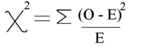
Using this formula Calculate Chi-square
Chi-square = 5.875
And degree of freedom is = n-1=7-1=6
Now let’s see the critical value from chi square distribution table at 5 % level of significance
So the critical value is 12.592
Since the Chi-Square calculated value is less than the critical value , we accept the null hypothesis and can conclude that the breakdowns are uniformly distributed.
Chi-Square Independence of Test
Use the test for independence to decide whether two variables (factors) are independent or dependent, i.e. whether these two variables have a significant association relationship between them or not . In this case there will be two qualitative survey questions or experiments and a contingency table will be constructed. The goal is to see if the two variables are unrelated (independent) or related (dependent). The null and alternative hypotheses are:
- H0: The two variables (factors) are independent.
- Ha: The two variables (factors) are dependent.
Let’s take an example
Example in which we want to investigate if gender and preferred color of shirt were independent. This means we want to find out if a person’s gender influences their color choice. We conducted a survey and organized the data in the table.
This table is observed values:
| Black | White | Red | Blue | |
| Male | 48 | 12 | 33 | 57 |
| Female | 34 | 46 | 42 | 26 |
Now first formulate null and alternative hypotheses
- H0: Gender and preferred shirt color are independent
- Ha: Gender and preferred shirt color are not independent
For calculating Chi-squared test statistics we need to calculate the expected value. So, add all the rows and columns and overall totals:
| Black | White | Red | Blue | Total | |
| Male | 48 | 12 | 33 | 57 | 150 |
| Female | 34 | 46 | 42 | 26 | 148 |
| Total | 82 | 58 | 75 | 83 | 298 |
After this we can calculate the expected value table from the above table for each entry using this formula = (row total * column total)/overall total
Expected value Table:
| Black | White | Red | Blue | |
| Male | 41.3 | 29.2 | 37.8 | 41.8 |
| Female | 40.7 | 28.8 | 37.2 | 41.2 |
Now calculate Chi square value using the formula for chi-Square Test:
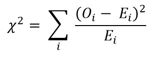
- Oi = Observed Value
- Ei = Expected Value
The value which we get is: Χ2 = 34.9572
Calculate Degree of Freedom
DF=(number of row-1)*(number of column-1)
Now find and compare the critical value to chi-square test statistic value:
To do this you can look up degree of freedom and the significance level (alpha) from the chi-square distribution table
At alpha =0.050, we will get critical value= 7.815
Since chi-square> critical value
Therefore, we reject the null hypothesis and we can conclude that gender and preferred shirt color are not independent.
Implementation of Chi- Square
Now , Let’s see the implementation of Chi- Square using some real life example in python:
- H0: Gender and preferred shirt color are independent
- Ha: Gender and preferred shirt color are not independent
Creating Dataset:
import pandas as pd
from scipy.stats import chi2_contingency
from scipy.stats import chi2


# Given dataset
df_dict = {
   'Black': [48, 34],
   'White': [12, 46],
   'Red': [33, 42],
   'Blue': [57, 26]
}
dataset_table = pd.DataFrame(df_dict, index=['Male', 'Female'])
print("Dataset Table:")
print(dataset_table)
print()


# Observed Values
Observed_Values = dataset_table.values
print("Observed Values:")
print(Observed_Values)
print()

# Perform chi-square test
val = chi2_contingency(dataset_table)
Expected_Values = val[3]
print("Expected Values:")
print(Expected_Values)
print()
# Degree of Freedom
no_of_rows = len(dataset_table.iloc[0:2, 0])
no_of_columns = 4
ddof = (no_of_rows - 1) * (no_of_columns - 1)
print("Degree of Freedom:", ddof)
print()
# Chi-square statistic
chi_square = sum([(o - e) ** 2. / e for o, e in zip(Observed_Values, Expected_Values)])
chi_square_statistic = chi_square[0] + chi_square[1]
print("Chi-square statistic:", chi_square_statistic)
print()
# Critical value
alpha = 0.05
critical_value = chi2.ppf(q=1-alpha, df=ddof)
print('Critical value:', critical_value)
print()
# p-value
p_value = 1 - chi2.cdf(x=chi_square_statistic, df=ddof)
print('p-value:', p_value)
print()
# Significance level
print('Significance level:', alpha)
print('p-value:', p_value)
print('Degree of Freedom:', ddof)
print()
# Hypothesis testing
if chi_square_statistic >= critical_value:
   print("Reject H0, Gender and preferred shirt color are independent")
else:
   print("Fail to reject H0, Gender and preferred shirt color are not independent")
print()
if p_value <= alpha:
   print("Reject H0, Gender and preferred shirt color are independent")
else:
   print("Fail to reject H0, Gender and preferred shirt color are not independent")
Output:

Mann- Whitney U Test
The Mann-Whitney U test serves as the non-parametric alternative to the independent sample t-test. It compares two sample means from the same population, determining if they are equal. This test is typically used for ordinal data or when assumptions of the t-test are not met.
The Mann-Whitney U test ranks all values from both groups together, then sums the ranks for each group. It calculates the test statistic, U, based on these ranks. The U-statistic is compared to a critical value from a table or calculated using an approximation. If the U-statistic is less than the critical value, the null hypothesis is rejected.
This is different from parametric tests like the t-test, which compare means and assume a normal distribution. The Mann-Whitney U test instead compares ranks and does not require the assumption of a normal distribution.
Understanding the Mann-Whitney U test can be difficult because the results are presented in group rank differences rather than group mean differences.
Formula for Mann-Whitney Test:
U= min(U1,U2)
Here,
- U= Mann-Whitney U Test
- n1= sample size one
- n2= sample size two
- R1= Rank of the sample size one
- R2= Rank of sample size 2
So, let’s understand this with a short example:
Suppose we want to compare the effectiveness of two different Treatment methods (Method A and Method B) in improving patients’ health. We have the following data:
- Method A: 3,4,2,6,2,5
- Method B: 9,7,5,10,6,8
Here, we can see that the data is not normally distributed, and the sample sizes are small.
Implementation of Mann-Whitney U test
Now, let’s perform the Mann-Whitney U test:
But first let’s formulate the Null and Alternative hypothesis
- H0: There is no difference between the Rank of each treatment
- Ha: There is a difference between the Rank of each treatment
Combine all the treatments: 3,4,2,6,2,5,9,7,5,10,6,8
Sorted data : 2,2,3,4,5,5,6,6,7,8,9,10
Rank of sorted data: 1,2,3,4,5,6,7,8,9,10,11,12
- Ranking the Data Separately:
- Method A: 3(3),4(4),2(1.5),6(7.5),2(1.5),5(5.5)
- Method B: 9(11),7(9),5(5.5),10(12),6(1.5),8(10)
- Calculating sum of rank):
- R1: 3+4+1.5+7.5+1.5+5.5=23
- R2: 11+9+5.5+12+1.5+10=55
Now calculate the statistic value using this formula:
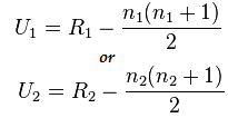
Here n1=6 and n2=6
And the value after calculation for U1=2 and for U2= 34
Calculating U statistic :
Us= min(U1,U2)= min(2,34)= 2
From Mann-Whitney Table we can find the critical value
In this case Critical Value will be 5
Since Uc= 5 which is greater than Us at 5% level of significance .So, we reject H0
Hence we can conclude that there is a difference between the Rank of each treatment.
Implementation with python
from scipy.stats import mannwhitneyu, norm
import numpy as np
TreatmentA = np.array([3,4,2,6,2,5])
TreatmentB = np.array([9,7,5,10,6,8])

# Perform Mann-Whitney U test
U_statistic, p_value = mannwhitneyu(TreatmentA, TreatmentB)

# Print the result
print(f'The U-statistic is {U_statistic:.2f} and the p-value is {p_value:.4f}')

if p_value < 0.05:
   print("Reject Null Hypothesis: There is a significant difference between the Rank of each treatment.")

else:
   print("Fail to Reject Null Hypothesis: Fail to Reject Null Hypothesis: There is no enough evidence to conclude that  there is  difference between the Rank of each treatment")
Output:

Kruskal –Wallis Test
Kruskal –Wallis Test is used with multiple groups. It is the non-parametric and a valuable alternative to a one-way ANOVA test when the normality and equality of variance assumptions are violated. Kruskal –Wallis Test compares medians of more than two independent groups.
It tests the Null Hypothesis when k independent samples (k>=3) are drawn from a population with identical distributions, without requiring the condition of normality for the populations.
Assumptions:
Ensure there are at least three independently drawn random samples. Each sample has at least 5 observations, n>=5
Consider an example where we want to determine if the studying technique used by three groups of students affects their exam scores. We can use the Kruskal-Wallis Test to analyze the data and assess whether there are statistically significant differences in exam scores among the groups.
Formulate the null hypothesis for this as:
- H0: There is no difference in exam scores among the three groups of students.
- Ha: There is a difference in exam scores among the three groups of students.
Wilcoxon Signed Rank Test
Wilcoxon Signed Rank Test (also known as Wilcoxon Matched Pair Test) is the non-parametric version of dependent sample t-test or paired sample t-test. Sign test is the other nonparametric alternative to the paired sample t-test. It is used when the variables of interest are dichotomous in nature (such as Male and Female, Yes and No). Wilcoxon Signed Rank Test is also a nonparametric version for one sample t-test. Wilcoxon Signed Rank Test compares the medians of the groups under two situations (paired samples) or it compares the median of the group with hypothesized median (one sample).
Let’s understand this with an example suppose we have data on the daily cigarette consumption of smokers before and after participating in a 8-week program and we want to determine if there is a significant difference in daily cigarette consumption before and after the program then we will use this test
The hypothesis formulation for this will be
- H0: There is no difference in daily cigarette consumption before and after the program.
- Ha: There is a difference in daily cigarette consumption before and after the program
Test for Normality
Let us now discuss Normality tests:
Shapiro Wilk test
The Shapiro-Wilk test assesses whether a given sample of data comes from a normally distributed population. It’s one of the most commonly used tests for checking normality. The test is particularly useful when dealing with relatively small sample sizes.
In the Shapiro-Wilk test:
- Null Hypothesis : The sample data comes from a population that follows a normal distribution.
- Alternative Hypothesis : The sample data does not come from a population that follows a normal distribution.
The test statistic generated by the Shapiro-Wilk test measures the discrepancy between the observed data and the expected data under the assumption of normality. If the p-value associated with the test statistic is less than a chosen significance level (e.g., 0.05), we reject the null hypothesis, indicating that the data are not normally distributed. If the p-value is greater than the significance level, we fail to reject the null hypothesis, suggesting that the data may follow a normal distribution.
First Let’s Create a dataset for these test you can use any dataset of your choice:
import pandas as pd
# Create the dictionary with the provided data
data = {
    'population': [6.1101, 5.5277, 8.5186, 7.0032, 5.8598],
    'profit': [17.5920, 9.1302, 13.6620, 11.8540, 6.8233]
}

# Create the DataFrame
df = pd.DataFrame(data)
response_var=df['profit']

Here, a sample for running Shapiro -Wilk test on python:
from scipy.stats import shapiro
stat, p_val = shapiro(response_var)
print(f'Shapiro-Wilk Test: Statistic={stat} p-value={p_val}')

if p_val > alpha:
    print('Data looks normal (fail to reject H0)')

else:
    print('Data looks normal (fail to reject H0)')
Output:

This test is most appropriate for relatively small sample sizes( n=< 50-2000) as it becomes less reliable with larger sample sizes.
Anderson-Darling
It assesses whether a given sample of data comes from a specified distribution, such as the normal distribution. It’s similar to the Shapiro-Wilk test but is more sensitive especially for smaller sample sizes.
It suits several distributions, including the normal distribution, for cases where the parameters of the distribution are unknown.
Here, Python code for Implementing it:
from scipy.stats import anderson
response_var = data['profit']
alpha = 0.05

# Anderson-Darling Test
result = anderson(response_var)
print(f'Anderson statistics: {result.statistic:.3f}')
if result.statistic > result.critical_values[-1]:
   p_value = 0.0  # The p-value is essentially 0 if the statistic exceeds the largest critical value

else:
   p_value = result.significance_level[result.statistic < result.critical_values][-1]

print("P-value:", p_value)
if p_value < alpha:
   print("Reject null hypothesis: Data does not look normally distributed")

else:
   print("Fail to reject null hypothesis: Data looks normally distributed")
Output:

Jarque-Bera Test
The Jarque-Bera test assesses whether a given sample of data comes from a normally distributed population. It is based on the skewness and kurtosis of the data.
Here’s the implementation of Jarque-Bera Test in Python with sample data:
from scipy.stats import jarque_bera
# Performing Jarque-Bera test
test_statistic, p_value = jarque_bera(response_var)
print("Jarque-Bera Test Statistic:", test_statistic)
print("P-value:", p_value)
# Interpreting results
alpha = 0.05
if p_value < alpha:
   print("Reject null hypothesis: Data does not look normally distributed")

else:
   print("Fail to reject null hypothesis: Data looks normally distributed")
Output:

| Category | Parametric Statistical Techniques | Non- parametric StatisticalTechniques |
| correlation | Pearson Product Moment Coefficient of Correlation (r) | Spearman Rank Coefficient Correlation (Rho), Kendall‟s Tau |
| Two groups, independent measures | Independent t-test | Mann-Whitney U test |
| More than two groups, independent measures | One-way ANOVA | Kruskal-Wallis one way ANOVA |
| Two groups, repeated measures | Paired t-test | Wilcoxon matched pair signed rank test |
| More than two groups, repeated measures | One-way, repeated measures ANOVA | Friedman’s two way Analysis of Variance |
Conclusion
Hypothesis testing is essential for evaluating claims about population parameters using sample data. Parametric tests rely on specific assumptions and are suitable for interval or ratio data, while non-parametric tests are more flexible and applicable to nominal or ordinal data without strict distributional assumptions. Tests such as Shapiro-Wilk and Anderson-Darling assess normality, while Chi-square and Jarque-Bera evaluate goodness of fit. Understanding the differences between parametric and non-parametric tests is crucial for selecting the appropriate statistical approach. Overall, hypothesis testing provides a systematic framework for making data-driven decisions and drawing reliable conclusions from empirical evidence.
Ready to master advanced statistical analysis? Enroll in our BlackBelt Data Analysis course today! Gain expertise in hypothesis testing, parametric and non-parametric tests, Python implementation, and more. Elevate your statistical skills and excel in data-driven decision-making. Join now!
Frequently Asked Questions
A. Parametric tests make assumptions about the population distribution and parameters, such as normality and homogeneity of variance, whereas non-parametric tests do not rely on these assumptions. Parametric tests have more power when assumptions are met, while non-parametric tests are more robust and applicable in a wider range of situations, including when data are skewed or not normally distributed.
A. The chi-square test is used to determine whether there is a significant association between two categorical variables. It commonly analyzes categorical data and tests hypotheses about the independence of variables in contingency tables.
A. The Mann-Whitney U test compares two independent groups when the dependent variable is ordinal or not normally distributed. It assesses whether there is a significant difference between the medians of the two groups.
A. The Shapiro-Wilk test assesses whether a sample comes from a normally distributed population. It tests the null hypothesis that the data follow a normal distribution. If the p-value is less than the chosen significance level (e.g., 0.05), we reject the null hypothesis, concluding that the data are not normally distributed.


